
You are here: Start » Machine Vision Guide » Image Processing
Image Processing
Introduction
There are two major goals of Image Processing techniques:
- To enhance an image for better human perception
- To make the information it contains more salient or easier to extract
It should be kept in mind that in the context of computer vision only the second point is important. Preparing images for human perception is not part of computer vision; it is only part of information visualization. In typical machine vision applications this comes only at the end of the program and usually does not pose any problem.
The first and the most important advice for machine vision engineers is: avoid image transformations designed for human perception when the goal is to extract information. Most notable examples of transformations that are not only not interesting, but can even be highly disruptive, are:
- JPEG compression (creates artifacts not visible by human eye, but disruptive for algorithms)
- CIE Lab and CIE XYZ color spaces (specifically designed for human perception)
- Edge enhancement filters (which improve only the "apparent sharpness")
- Image thresholding performed before edge detection (precludes sub-pixel precision)
Examples of image processing operations that can really improve information extraction are:
- Gaussian image smoothing (removes noise, while preserving information about local features)
- Image morphology (can remove unwanted details)
- Gradient and high-pass filters (highlight information about object contours)
- Basic color space transformations like HSV (separate information about chromaticity and brightness)
- Pixel-by-pixel image composition (e.g. can highlight image differences in relation to a reference image)
Regions of Interest
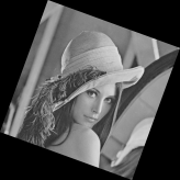
The image processing tools provided by Adaptive Vision have a special inRoi input (of Region type), that can limit the spatial scope of the operation. The region can be of any shape.
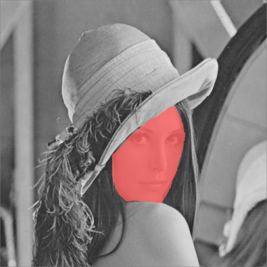
An input image and the inRoi. |
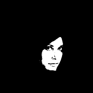
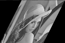
Result of an operation performed within inRoi. |
Remarks:
- The output image will be black outside of the inRoi region.
- To obtain an image that has its pixels modified in inRoi and copied outside of it, one can use the ComposeImages filter.
- The default value for inRoi is Auto and causes the entire image to be processed.
- Although inRoi can be used to significantly speed up processing, it should be used with care. The performance gain may be far from proportional to the inRoi area, especially in comparison to processing the entire image (Auto). This is due to the fact, that in many cases more SSE optimizations are possible when inRoi is not used.
Some filters have a second region of interest called inSourceRoi. While inRoi defines the range of pixels that will be written in the output image, the inSourceRoi parameter defines the range of pixels that can be read from the input image.
Image Boundary Processing
Some image processing filters, especially those from the Image Local Transforms category, use information from some local neighborhood of a pixel. This causes a problem near the image borders as not all input data is available. The policy applied in our tools is:
- Never assume any specific value outside of the image, unless specifically defined by the user.
- If only partial information is available, it is better not to detect anything, than detect something that does not exist.
In particular, the filters that use information from a local neighborhood just use smaller (cropped) neighbourhood near the image borders. This is something, however, that has to be taken into account, when relying on the results – for example results of the smoothing filters can be up to 2 times less smooth at the image borders (due to half of the neighborhood size), whereas results of the morphological filters may "stick" to the image borders. If the highest reliability is required, the general rule is: use appropriate regions of interest to ignore image processing results that come from incomplete information (near the image borders).
Toolset
Image Combinators
The filters from the Image Combinators category take two images and perform a pixel-by-pixel transformation into a single image. This can be used for example to highlight differences between images or to normalize brightness – as in the example below:
Input image with high reflections. |
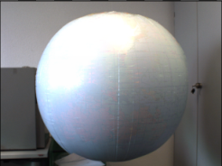
Image of the reflections (calibrating). |
The result of applying DivideImages with inScale = 128 (inRoi was used). |
Image Smoothing
The main purpose of the image smoothing filters (located in the Image Local Transforms category) is removal of noise. There are several different ways to perform this task with different trade-offs. On the example below three methods are presented:
- Mean smoothing – simply takes the average pixel value from a rectangular neighborhood; it is the fastest method.
- Median smoothing – simply takes the median pixel value from a rectangular neighborhood; preserves edges, but is relatively slow.
- Gauss smoothing – computes a weighted average of the pixel values with Gaussian coefficients as the weights; its advantage is isotropy and reasonable speed for small kernels.
Input image with some noise. |

Result of applying SmoothImage_Mean. |

Result of applying SmoothImage_Gauss. |

Result of applying SmoothImage_Median. |
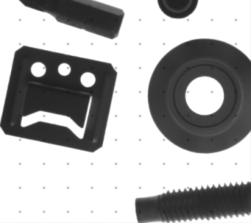
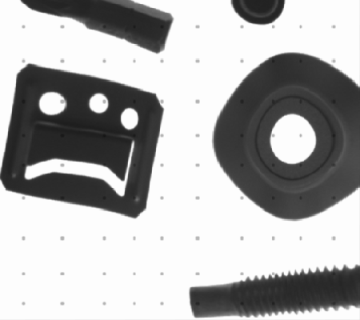
Image Morphology
Basic morphological operators – DilateImage and ErodeImage – transform the input image by choosing maximum or minimum pixel values from a local neighborhood. Other morphological operators combine these two basic operations to perform more complex tasks. Here is an example of using the OpenImage filter to remove salt and pepper noise from an image:
Input image with salt-and-pepper noise. |

Result of applying OpenImage. |
Gradient Analysis
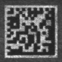
An image gradient is a vector describing direction and magnitude (strength) of local brightness changes. Gradients are used inside of many computer vision tools – for example in object contour detection, edge-based template matching and in barcode and DataMatrix detection.
Available filters:
- GradientImage – produces a 2-channel image of signed values; each pixel denotes a gradient vector.
- GradientMagnitudeImage – produces a single channel image of gradient magnitudes, i.e. the lengths of the vectors (or their approximations).
- GradientDirAndPresenceImage – produces a single channel image of gradient directions mapped into the range from 1 to 255; 0 means no significant gradient.
An input image. |
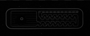
Result of GradientMagnitudeImage. |
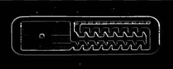
Result of GradientDirAndPresenceImage. |
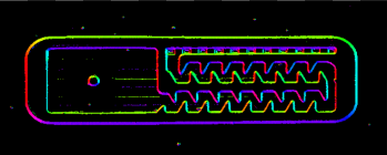
Diagnostic output of GradientImage showing hue-coded directions. |
Spatial Transforms
Spatial transforms modify an image by changing locations, but not values, of pixels. Here are sample results of some of the most basic operations:
Result of MirrorImage. |
Result of RotateImage. |
Result of ShearImage. |
Result of DownsampleImage. |
|
Result of TransposeImage. |
Result of TranslateImage. |
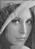
Result of CropImage. |
Result of UncropImage applied to the result of CropImage. |
There are also interesting spatial transform tools that allow to transform a two dimensional vision problem into a 1.5-dimensional one, which can be very useful for further processing:
An input image and a path.
Result of ImageAlongPath.
Spatial Transform Maps
The spatial transform tools perform a task that consist of two steps for each pixel:
- compute the destination coordinates (and some coefficients when interpolation is used),
- copy the pixel value.
In many cases the transformation is constant – for example we might be rotating an image always by the same angle. In such cases the first step – computing the coordinates and coefficients – can be done once, before the main loop of the program. Adaptive Vision provides the Image Spatial Transforms Maps category of filters for exactly that purpose. When you are able to compute the transform beforehand, storing it in the SpatialMap type, in the main loop only the RemapImage filter has to be executed. This approach will be much faster than using standard spatial transform tools.
The SpatialMap type is a map of image locations and their corresponding positions after given geometric transformation has been applied.
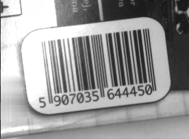
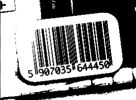
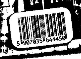
Additionally, the Image Spatial Transforms Maps category provides several filters that can be used to flatten the curvature of a physical object. They can be used for e.g. reading labels glued onto curved surfaces. These filters model basic 3D objects:
- Cylinder (CreateCylinderMap) – e.g. flattening of a bottle label.
- Sphere (CreateSphereMap) – e.g. reading a label from light bulb.
- Box (CreatePerspectiveMap_Points or CreatePerspectiveMap_Path) – e.g. reading a label from a box.
- Circular objects (polar transform) (CreateImagePolarTransformMap) - e.g. reading a label wrapped around a DVD disk center.
 |
 |
Example of remapping of a spherical object using CreateSphereMap and RemapImage. Image before and after remapping.
Furthermore custom spatial maps can be created with ConvertMatrixMapsToSpatialMap.
 |
 |
An example of custom image transform created with ConvertMatrixMapsToSpatialMap. Image before and after remapping.
Image Thresholding
The task of Image Thresholding filters is to classify image pixel values as foreground (white) or background (black). The basic filters ThresholdImage and ThresholdToRegion use just a simple range of pixel values – a pixel value is classified as foreground iff it belongs to the range. The ThresholdImage filter just transforms an image into another image, whereas the ThresholdToRegion filter creates a region corresponding to the foreground pixels. Other available filters allow more advanced classification:
- ThresholdImage_Dynamic and ThresholdToRegion_Dynamic use average local brightness to compensate global illumination variations.
- ThresholdImage_RGB and ThresholdToRegion_RGB select pixel values matching a range defined in the RGB (the standard) color space.
- ThresholdImage_HSx and ThresholdToRegion_HSx select pixel values matching a range defined in the HSx color space.
- ThresholdImage_Relative and ThresholdToRegion_Relative allow to use a different threshold value at each pixel location.
Input image with uneven light. |
Result of ThresholdImage – the bars can not be recognized. |
Result of ThresholdImage_Dynamic – the bars are correct. |
There is also an additional filter SelectThresholdValue which implements a number of methods for automatic threshold value selection. It should, however, be used with much care, because there is no universal method that works in all cases and even a method that works well for a particular case might fail in special cases.
Image Pixel Analysis
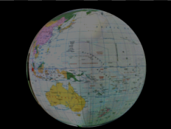
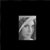
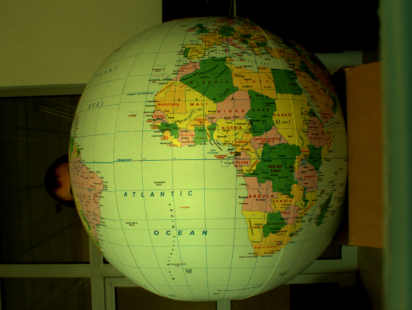
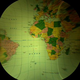
When reliable object detection by color analysis is required, there are two filters that can be useful: ColorDistance and ColorDistanceImage. These filters compare colors in the RGB space, but internally separate analysis of brightness and chromaticity. This separation is very important, because in many cases variations in brightness are much higher than variations in chromaticity. Assigning more significance to the latter (high value of the inChromaAmount input) allows to detect areas having the specified color even in presence of highly uneven illumination:
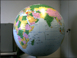
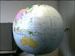
Input image with uneven light. |
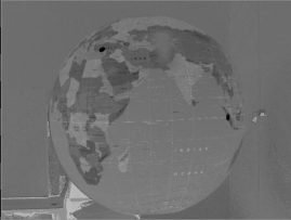
Result of ColorDistanceImage for the red color with inChromaAmount = 1.0. Dark areas correspond to low color distance. |
Result of thresholding reveals the location of the red dots on the globe. |
Image Features
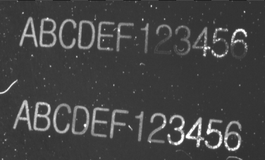
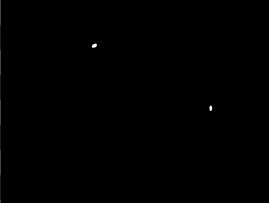
Image Features is a category of image processing tools that are already very close to computer vision – they transform pixel information into simple higher-level data structures. Most notable examples are: ImageLocalMaxima which finds the points at which the brightness is locally the highest, ImageProjection which creates a profile from sums of pixel values in columns or in rows, ImageAverage which averages pixel values in the entire region of interest. Here is an example application:
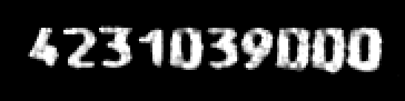
Input image with digits to be segmented. |

Result of preprocessing with CloseImage. |
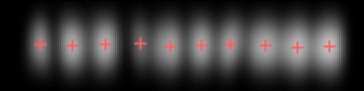
Digit locations extracted by applying SmoothImage_Gauss and ImageLocalMaxima. |

Profile of the vertical projection revealing regions of digits and the boundaries between them. |
| Previous: Machine Vision Guide | Next: Blob Analysis |