
You are here: Start » Machine Vision Guide » 1D Edge Detection
1D Edge Detection
Introduction
1D Edge Detection (also called 1D Measurement) is a classic technique of machine vision where the information about image is extracted from one-dimensional profiles of image brightness. As we will see, it can be used for measurements as well as for positioning of the inspected objects.
Main advantages of this technique include sub-pixel precision and high performance.
Concept
The 1D Edge Detection technique is based on an observation that any edge in the image corresponds to a rapid brightness change in the direction perpendicular to that edge. Therefore, to detect the image edges we can scan the image along a path and look for the places of significant change of intensity in the extracted brightness profile.
The computation proceeds in the following steps:
- Profile extraction – firstly the profile of brightness along the given path is extracted. Usually the profile is smoothed to remove the noise.
- Edge extraction – the points of significant change of profile brightness are identified as edge points – points where perpendicular edges intersect the scan line.
- Post-processing – the final results are computed using one of the available methods. For instance ScanSingleEdge filter will select and return the strongest of the extracted edges, while ScanMultipleEdges filter will return all of them.
Example
 |
 |
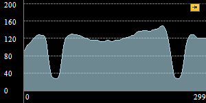 |
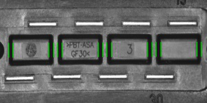
The image is scanned along the path and the brightness profile is extracted and smoothed.
 |
 |
 |
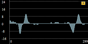
Brightness profile is differentiated. Notice four peaks of the profile derivative which correspond to four prominent image edges intersecting the scan line. Finally the peaks stronger than some selected value (here minimal strength is set to 5) are identified as edge points.
Filter Toolset
Basic toolset for the 1D Edge Detection-based techniques scanning for edges consists of 9 filters each of which runs a single scan along the given path (inScanPath). The filters differ on the structure of interest (edges / ridges / stripes (edge pairs)) and its cardinality (one / any fixed number / unknown number).
| Edges | |
|---|---|
| Single Result |  |
| Multiple Results |  |
| Fixed Number of Results |  |
| Stripes | |
|---|---|
| Single Result | 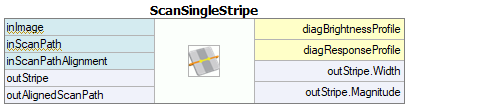 |
| Multiple Results | 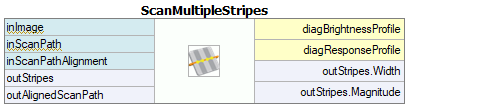 |
| Fixed Number of Results | 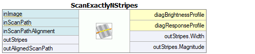 |
| Ridges | |
|---|---|
| Single Result | 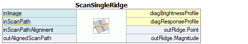 |
| Multiple Results | 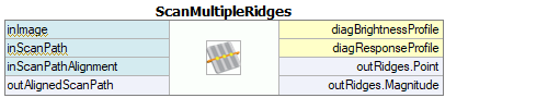 |
| Fixed Number of Results | 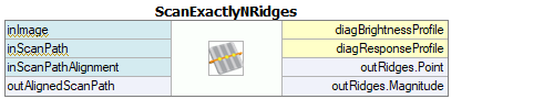 |
Note that in Adaptive Vision Library there is the CreateScanMap function that has to be used before a usage of any other 1D Edge Detection function. The special function creates a scan map, which is passed as an input to other functions considerably speeding up the computations.
Parameters
Profile Extraction

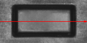
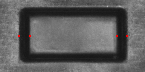
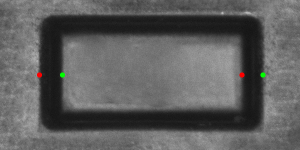
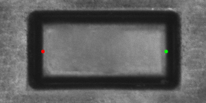
In each of the nine filters the brightness profile is extracted in exactly the same way. The stripe of pixels along inScanPath of width inScanWidth is traversed and the pixel values across the path are accumulated to form one-dimensional profile. In the picture on the right the stripe of processed pixels is marked in orange, while inScanPath is marked in red.
The extracted profile is smoothed using Gaussian smoothing with standard deviation of inSmoothingStdDev. This parameter is important for the robustness of the computation - we should pick the value that is high enough to eliminate noise that could introduce false / irrelevant extrema to the profile derivative, but low enough to preserve the actual edges we are to detect.
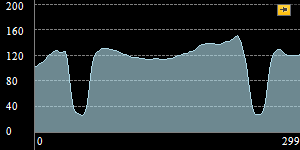
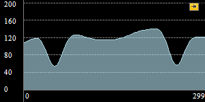
The inSmoothingStdDev parameter should be adjusted through interactive experimentation using diagBrightnessProfile output, as demonstrated below.
 |
 |
 |
Too low inSmoothingStdDev - too much noise |
Appropriate inSmoothingStdDev - low noise, significant edges are preserved |
Too high inSmoothingStdDev - significant edges are attenuated |
Edge Extraction
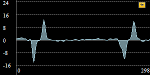
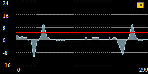
After the brightness profile is extracted and refined, the derivative of the profile is computed and its local extrema of magnitude at least inMinMagnitude are identified as edge points. The inMinMagnitude parameter should be adjusted using the diagResponseProfile output.
The picture on the right depicts an example diagResponseProfile profile. In this case the significant extrema vary in magnitude from 11 to 13, while the magnitude of other extrema is lower than 3. Therefore any inMinMagnitude value in range (4, 10) would be appropriate.
Edge Transition
Filters being discussed are capable of filtering the edges depending on the kind of transition they represent - that is, depending on whether the intensity changes from bright to dark, or from dark to bright. The filters detecting individual edges apply the same condition defined using the inTransition parameter to each edge (possible choices are bright-to-dark, dark-to-bright and any).
inTransition = Any |
inTransition = BrightToDark |
inTransition = DarkToBright |
Stripe Intensity
The filters detecting stripes expect the edges to alternate in their characteristics. The parameter inIntensity defines whether each stripe should bound the area that is brighter, or darker than the surrounding space.
 inIntensity = Dark |
 inIntensity = Bright |
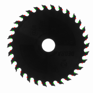
Case Study: Blades
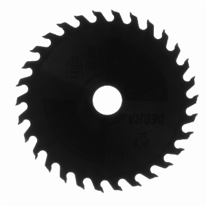
Assume we want to count the blades of a circular saw from the picture.
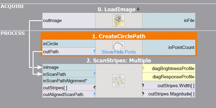
We will solve this problem running a single 1D Edge Detection scan along a circular path intersecting the blades, and therefore we need to produce appropriate circular path. For that we will use a straightforward CreateCirclePath filter. The built-in editor will allow us to point & click the required inCircle parameter.
The next step will be to pick a suitable measuring filter. Because the path will alternate between dark blades and white background, we will use a filter that is capable of measuring stripes. As we do not now how many blades there are on the image (that is what we need to compute), the ScanMultipleStripes filter will be a perfect choice.
We expect the measuring filter to identify each blade as a single stripe (or each space between blades, depending on our selection of inIntensity), therefore all we need to do to compute the number of blades is to read the value of the outStripes.Count property output of the measuring filter.
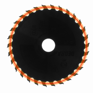
The program solves the problem as expected (perhaps after increasing the inSmoothingStdDev from default of 0.6 to bigger value of 1.0 or 2.0) and detects all 30 blades of the saw.
 |
 |
| Previous: Blob Analysis | Next: 1D Edge Detection – Subpixel Precision |