You are here: Start » Machine Vision Guide » Deep Learning

Deep Learning

Table of contents:

1. Overview
2. Anomalies detection
3. Features detection (segmentation)
4. Object classification
5. Troubleshooting

1. Overview

Deep Learning is a milestone machine learning technique in computer vision that enables the user to easily solve a wide range computer vision problems using features learned from training data.

Main advantages of this technique are: simple configuration, short development time, versatility of possible applications and high performance.

Using deep learning functionality includes two stages:

1. training the model - automatically generating a model based on features learned from training examples,
2. using the model - applying the model to new images in order to perform certain machine vision tasks.

Applications:

• detection of surface defects: cracks, damages or discoloration,
• detection of shape defects: redundant elements, missing parts, shape deformations,
• advanced edge localization,
• finding defects in object patterns,
• quality analysis of objects with variable shape,
• separation, sorting, matching and identification of objects with respect to predefined classes.

Available Deep Learning applications

1. Anomalies detection - This technique is used to detect samples with any potential defects, deformations, anomalies or damage. It only needs a set of fault-free samples to learn the normal appearance and several faulty ones to define the level of tolerable variations.


An example of anomalies detection. This tool is useful especially in cases where defects are unknown or too difficult to define upfront.

2. Features detection (segmentation) - This technique is used to precisely segment one or more classes of features within an image. The pixels belonging to each class must be marked by the user in the first step. The result of this technique is an array of probability maps for every class.


An example of image segmentation. This technique was created to precisely segment any elements on images.

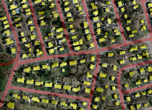
3. Object classification - This technique is used to identify affiliation of object to one of predefined classes. First, it is necessary to provide images which represent the classes. The result of this technique is an assignment of image to one of the classes with indicated confidence of classification.


An example of image classification. This technique was created to accurately identify class of object in the image.

Basic terminology

The users do not have to be equipped with the specialistic scientific knowledge to design their own deep learning solutions. However, it may be very useful to understand the basic terminology and principles behind the process.

Deep neural networks

Adaptive Vision gives access to deep convolutional neural networks architectures created, adjusted and tested to solve industrial-grade machine vision tasks. Each network is a set of trainable convolutional filters and neural connections which can model complex transformations of the image to extract relevant features and use them in order to solve particular problem. However, they are useless without proper amount of good quality data provided for training process (adjusting weights of filters and connections). This documentation gives necessary practical hints on preparing an effective deep learning model.

Due to various levels of tasks complexity and different expected execution times, the users can choose one of five available network depths. The Network depth parameter is an abstract value defining the memory capacity of the network (i.e., the number of layers and filters of a network) and ability to solve more complex problems. The list below gives hints about selecting the proper depth for a task characteristics and conditions.

1. Low depth (value 1-2)

   • a problem is simple to define,
   • a problem could be easily solved by a human inspector,
   • a short time of execution is required,
   • background and lightning do not change across images,
   • well-positioned objects and good quality of images.

2. Standard depth (default, value 3)

   • suitable for a majority of applications without any special conditions,
   • a modern CUDA-enabled GPU is available.

3. High depth (value 4-5)

   • a big amount of training data is available,
   • a problem is hard or very complex to define and solve,
   • complicated irregular patterns across images,
   • long training and execution times are not a problem,
   • a large amount of GPU RAM (≥6GB) is available,
   • varying background, lightning and/or positioning of objects.

Tip: test your solution with a lower depth first, and then increase it if needed.

Note: a higher network depth will lead to a significant increase in memory and computational complexity of training and execution.

Training

Model training is an iterative process of updating neural network weights based on the training data. One iteration involves some number of steps (determined automatically), each step consists of the following operations:

1. selection of a small subset (batch) of training samples,
2. calculation of network error for these samples,
3. updating weights to achieve lower error for these samples.

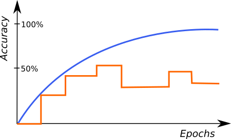
At the end of each iteration, the current model is evaluated on a separate set of validation samples selected before the training process. Validation set is automatically chosen from the training samples. It is used to simulate how neural network would work with real images not used during training. Only a set of network weights corresponding with the best validation score at the end of training is saved as the final solution. Monitoring the training and validation score (blue and orange lines in the figures below) in consecutive iterations gives fundamental information about the progress:

1. both training and validation scores are improving - keep training, model can still improve,
2. both training and validation scores has stopped improving - keep training for a few iterations more and stop if still no change,
3. training score is improving, but validation score has stopped or is going worse - you can stop training, model has probably started overfitting your training data (remembering exact samples rather than learning rules about features). It may be caused by too small amount of diverse samples or too low complexity of problem for a network selected.

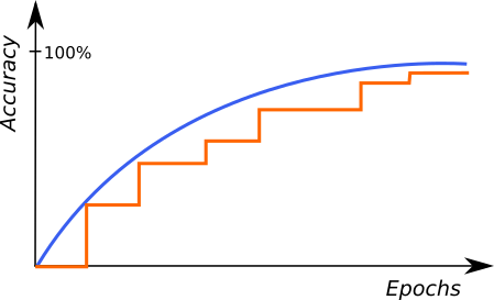
An example of correct training.

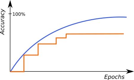
A graph characteristic for network overfitting.

Above graphs represent training progress in our Deep Learning Editor, the blue line indicates the performance on training samples, and the orange line represents the performance on validation samples. Please note the blue line is plotted more frequently than the orange line, as validation performance is verified only at the end of each iteration.

Preprocessing

To adjust the performance on your particular task, the user can apply some additional transformations to input images before training starts:

1. Downsample ― reduction of image size to accelerate training and execution times at the expense of lower level of details possible to detect. Increasing this parameter by 1 will result in downsampling by the factor of 2 over both image dimension.
2. Convert to grayscale ― while working with problems where color does not matter, you can choose to work with monochrome versions of images.

Augmentation

In case when the number of training images can be too small to represent all possible variations of samples, it is recommended to use data augmentation that adds artificially modified samples during training. This option can also help avoiding overfitting.

Available augmentations are (please note that some augmentations are not available for all networks):

1. Luminance ― if greater than 0% samples with random image brightness changes will be added. The value of the parameter defines the percentage range of maximum brightness changes (both darker and brighter) relatively to the full image range.
2. Noise ― if greater than 0% samples with random uniform noise will be added. Each channel and pixel is modified separately in the range defined by percentage of the full image range.
3. Rotation ― if greater than 0 randomly rotated (by ± parameter value degrees) samples will be added.
4. Flip Up-Down ― if enabled samples reflected along the X axis will be added.
5. Flip Left-Right ― if enabled samples reflected along the Y axis will be added.

Warning: the choice of augmentation options depends only on the task we want to solve, sometimes they might be harmful for quality of a solution. For simple example, enabling the Rotation should not be used if the rotations are not expected in a production environment. Enabling augmentations also increases the network training time (but does not affect execution time!)

2. Anomalies detection

This technique tries to find any images that significantly deviate from normal image appearance learned during training phase. It is done by examining the "deviation" of a test image from a "correct image" claimed by the network. If the overall deviation score exceeds a given threshold, the image is marked as defected. The suggested threshold is automatically calculated after the training phase but can be adjusted by user in the Deep Learning Editor using the interactive histogram tool described below.

Interactive histogram tool

After the training phase, scores are calculated for every training sample and presented in the form of histogram; good samples are marked with green, bad samples with red bars. In the perfect case, the deviation of good samples should be close to 0, and for bad samples around 10 or higher. In reality, these values may be different and can change depending on the case. In order to achieve more robust threshold, it is recommended to perform training with a large number of samples from both groups. When we operate on a limited number of samples, the determined threshold may be unsure. For this reason, our software allows to define uncertainty area with additional thresholds in order to receive information about the confidence of a model during execution.

The histogram tool where green bars represent correct images and red bars represent defected images and their deviation scores. T marks the main threshold and T1, T2 define the area of uncertainty.

If there is no (or very narrow) space between bars for good and bad samples it suggest poor model accuracy. It may be caused by too complicated or poorly defined task or wrong training parameters.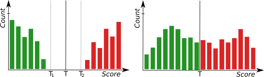

On the left: a histogram presenting well-separated groups. On the right: a model with poor accuracy.

Defect heatmaps

The maps of deviations for each pixel (called Heatmap) and the "correct images" claimed by network are available as filter outputs for further processing.

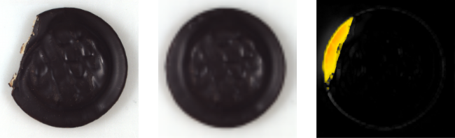
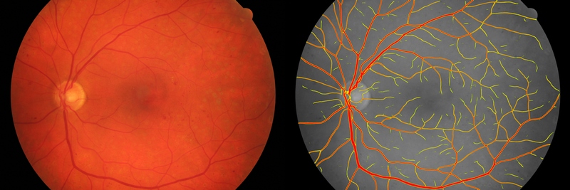
From left to right: An input image, corresponding "correct image" predicted by network and corresponding heatmap of defects

Network architectures

Adaptive Vision offers below types of network architecture suitable for defect detection.

Local network

A network type analyzing the image in fragments of size determined by Feature size parameter (description in the next section). Recommended for relatively small defects, irregular patterns and local appearance changes.

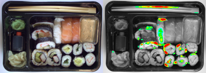
An example of complex defects detection inside a sushi box.

Global network

A network type analyzing the entire image context. Recommended for detection of large defects, deformations and missing objects. The main advantage of this network is a short time of training and execution.

An example of cookie shape defects detection.

Texture network

A network type focused on analyzing repeatable textures and regular patterns. Recommended for detection of both small and large defects in textiles and surfaces. Characterized by a long training time but very precise heatmaps.

An example of defects detection in a cloth.

Feature size

This parameter defines the expected defect size in pixels for Local and Texture networks. The value should be large enough so that the minimal defect would take around 1/3 of its size. Increasing this parameter will significantly increase the time required for training, but it usually leads to a better quality of results. However, sometimes it may be hard to choose the value that works well for both small and large defects and the only way is to prepare separate models.

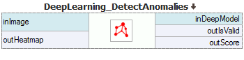
Model usage

Use DeepLearning_DetectAnomalies filter.

3. Feature detection (segmentation)

This technique is used to precisely segment one or more classes of features or objects within an image. The pixels belonging to each class must be marked by the user in the first step. The result of this technique is an array of probability maps for every class.

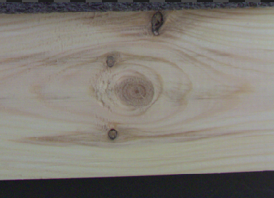
Original image.

Found knots.

Preparing the data

The most important task for the user is to prepare defects/class masks and choose an appropriate feature size before training. A defects (class) mask contains pixels indicating which regions of the input image represent a given feature.

Marked knots.

Marked cracks.

Feature size relates to the size of a defect we intend to detect. The best results can be achieved when a feature size allows to contain a defect together with its immediate surroundings. In case when the selected feature size is too large, defects may be ignored by the network. However, a feature size that is too small may cause the algorithm to find only the inside of a defect and not its edges.

You can use an intuitive editor available with Adaptive Vision Studio to prepare a Deep Learning model.

Editor for marking defects.

Tip: To accelerate training you can limit ROI to make it fit to the size of a defect. It will prevent the algorithm from unnecessarily analyzing the same background in multiple images, but at least one image in training set must contain whole background in region of interest.

Notice: All defects should be marked on all training images, or ROI should be limited to include only marked defects. When training data includes both marked and unmarked defects, it creates inconsistency, which reduces the quality of training.

Multiple defect classes

Feature detection (segmentation) allows the user to define multiple defect classes. For example you can separate material discoloration from surface scratches using one model.

The above image shows two masks applied to the input image.

Tip: In case when two class masks overlap each other, it may cause a conflict between classes over which class does the feature belongs to. In such situations both classes can be combined into one class or separate models should be used for those classes.

Notice: adding new features automatically increases network capacity, which may prolong the training process. Maximal number of features classes depends on your GPU card memory capacity.

Feature size

The best results should be achieved when a feature size allows to include a defect together with a part of its surroundings (context). A trained network examines the input image only by looking at it through windows defined by a feature size. For this reason, it is recommended to follow the rule that an operator, using the same context, should be able to properly decide whether a given sample contains a defect or not.

Accuracy tip: it is better to use larger than smaller feature size if you are not sure

Performance tip: a larger feature size increases the training time, it also needs more GPU memory and training samples to operate effectively. When feature size exceeds 96 pixels and still looks too small, it is worth considering the Downsample option.

Performance tip: if the execution time is not satisfying you can set the inOverlap filter input to False. It should speed up the inspection by 10 to 30% at the expense of less precise masks.

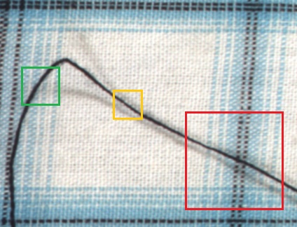
Examples of feature size: too large (red), optimal (green) and acceptable (orange). Remember that this is just a heuristic and can vary in some cases.

Model usage

Use DeepLearning_DetectFeatures filter to perform segmentation of features.

Parameters:

• To limit the area of image analysis you can use inRoi input.
• To increase segmentation precision you can use inOverlap option.
• Feature segmentation results are passed in a form of bit maps to outHeatmaps output as an array and outFeature1, outFeature2, outFeature3 and outFeature4 as separate images.

Notice: Enabling inOverlap option increases segmentation quality, but also prolongs feature segmentation process.

4. Object classification

This technique is used to identify class of object within an image.

Principle of operation

During the training, object classification learns the representation of user defined classes. Model uses generalized knowledge gained from samples provided for training, and aims to obtain good separation between classes.

Result of classification after training.

After the training is completed, user is presented with confusion matrix. It indicates, how well model separated user defined classes. It simplifies identification of model accuracy, when large number of samples is presented.

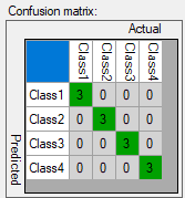
Confusion matrix presents assignment of samples to user defined classes.

Training parameters

Object classification has been designed to minimize the time needed to perform classification task on images provided by user. There are no additional parameters apart from default ones. List of parameters available for all Deep Learning algorithms.

Model usage

Use DeepLearning_ClassifyObject filter to perform classification.

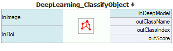
Parameters:

• To limit the area of image analysis you can use inRoi input.
• Classification results are passed to outClassName and outClassIndex outputs.
• Score value outScore indicates confidence of classification.

5. Troubleshooting

Below you will find a list of most common problems.

1. Network overfitting

A situation when network loses its ability to generalize over available problems and focuses only on test data.

Symptoms: during training, the validation graph stops at one level and training graph continues to rise. Defects on training images are marked very precisely, but defects on new images are marked poorly.

A graph characteristic for network overfitting.

Causes:

• The number of test samples is too small,
• Training time is too long.

Solution:

• Provide more real samples,
• Add more samples with possible object rotations.

2. Susceptibility to changes in lighting conditions.

Symptoms- network is not able to process images properly when even minor changes in lighting occur.

Causes:

• Samples with variable lighting were not provided.

Solution:

• Provide more samples with variable lighting,
• Enable "Luminance" option for automatic lighting augmentation.

3. No progress in network training.

Symptoms ― even though the training time is optimal, there is no visible training progress.

Training progress with contradictory samples.

Causes:

• The number of samples is too small or the samples are not variable enough,
• image contrast is too small,
• the chosen network architecture is too small,
• contradiction in defect masks.

Solution:

• Modify lighting to expose defects,
• Remove contradictions in defect masks.

Tip: Remember to mark all defects of a given type on the input images or remove images with unmarked defects. Marking only a part of defects of a given type may negatively influence the network learning process.

4. Training/sample evaluation is very slow

Symptoms ― training or sample evaluation takes a lot of time.

Causes:

• Resolution of the provided input images is too high,
• Fragments that cannot possibly contain defects are also analyzed.

Solution:

• Enable "Downsample" option to reduce the image resolution,
• Limit ROI for sample evaluation.

See also:

• Deep Learning Service Configuration - installation and configuration of Deep Learning service,
• Creating Deep Learning Model - how to use Deep Learning Editor.

Previous: Golden Template

Next: Common Filter Conventions