
You are here: Start » User Interface » Creating Deep Learning Model
Creating Deep Learning Model
Contents:
- Introduction
- Workflow
- Detecting anomalies 1
- Detecting anomalies 2
- Detecting features
- Classifying objects
- Segmenting instances
- Locating points
- Locating objects
- Tips and tricks
Introduction
Deep Learning editors are dedicated graphical user interfaces for DeepModel objects (which represent training results). Each time a user opens such an editor, he is able to add or remove images, adjust parameters and perform new training.
Since version 4.10 it is also an option to open a Deep Learning Editor as a stand-alone application, which is especially useful for re-training models with new images in production environment.
In 5.4 version the Aurora Vision Deep Learning tool-chain has been switched to a completely new training engine. Right now Feature Detection, Anomaly Detection 2, Object Classification, Point Location, Read Text and Locate Text are adopted to the new engine. The rest of the tools will be available soon.
Requirements:
- A Deep Learning license is required to use Deep Learning editors and filters.
- The Deep Learning Service must be up and running to perform model training.
Warning: Some of the Deep Learning algorithms, e.g. Instance Segmentation, require a lot of memory, therefore we highly recommend using the GPU version of Aurora Vision Deep Learning.
The currently available Deep Learning tools include:
- Anomaly Detection – for detecting unexpected object variations; trained with sample images marked simply as good or bad.
- Feature Detection – for detecting regions of defects (such as surface scratches) or features (such as vessels on medical images); trained with sample images accompanied by precisely marked ground-truth regions.
- Object Classification – for identifying the name or the class of the most prominent object on an input image; trained with sample images accompanied by the expected class labels.
- Instance Segmentation – for simultaneously locating, segmenting and classifying multiple objects in an image; trained with sample images accompanied by precisely marked regions of each individual object.
- Point Location – for locating and classifying multiple key points; trained with sample images accompanied by marked points of expected classes.
- Read Characters – for locating and classifying multiple characters; this tool uses a pretrained model and cannot be manually retrained by a user, so it is not elaborated upon further in this entry.
- Text Location – for locating text; this tool uses a pretrained model and cannot be manually retrained by a user, so it is not elaborated upon further in this entry.
- Object Location – for locating and classifying multiple objects; trained with sample images accompanied by marked bounding rectangles of expected classes.
Technical details about these tools are available at Machine Vision Guide: Deep Learning while this article focuses on the training graphical user interface.
Workflow
You can open a Deep Learning Editor via:
- a filter in Aurora Vision Studio:
- Place the relevant DL filter (e.g. DL_DetectFeatures or DL_DetectFeatures_Deploy) in the Program Editor.
- Go to its Properties.
- Click on the button next to the inModelDirectory or inModelId.ModelDirectory parameter.
- a standalone Deep Learning Editor application:
- Open a standalone Deep Learning Editor application (which can be found in the Aurora Vision Studio installation folder as "DeepLearningEditor.exe", in Aurora Vision folder in Start menu or in Aurora Vision Studio application in Tools menu).
- Choose whether you want to create a new model or use an existing one:
- Creating a new model: Select the relevant tool for your model and press OK, then select or create a new folder where files for your model will be contained and press OK.
- Choosing existing model: Navigate to the folder containing your model files – either write a path to it, click on the button next to field to browse to it or select one of the recent paths if there are any; then press OK.
The Deep Learning model preparation process is usually split into the following steps:
- Loading images – load training images from disk.
- Labeling images – mark features or attach labels on each training image.
- Assigning image sets – allocate images to train, test or validation set.
- Setting the region of interest (optional) – select the area of the image to be analyzed.
- Adjusting training parameters – select training parameters, preprocessing steps and augmentations specific for the application at hand.
- Training the model and analyzing results.
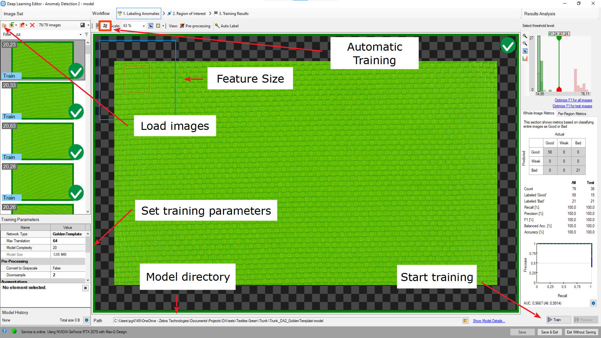
Overview of a Deep Learning Editor.
Important features:
- Pre-processing button – located in the top toolbar; allows you to see the changes applied to a training image e.g. grayscale or downsampling.
- Current Model directory – located in the bottom toolbar; allows you to switch a model being in another directory or to simply see which model you are actually working on.
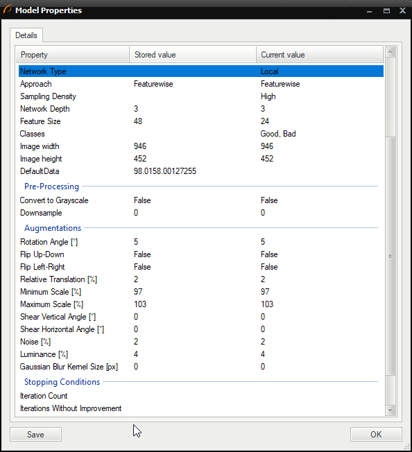
- Show Model Details button – located next to the previous control; allows you to display information on the current model and save them to a file.
- Train & Resume buttons – allow you to start training or resume it in case you have changed some of training parameters.
- Saving buttons:
- Save – saves the current model in chosen location.
- Save & Exit – saves the model and then exits the Deep Learning Editor.
- Exit Without Saving – exits the editor, but the model is not being saved.
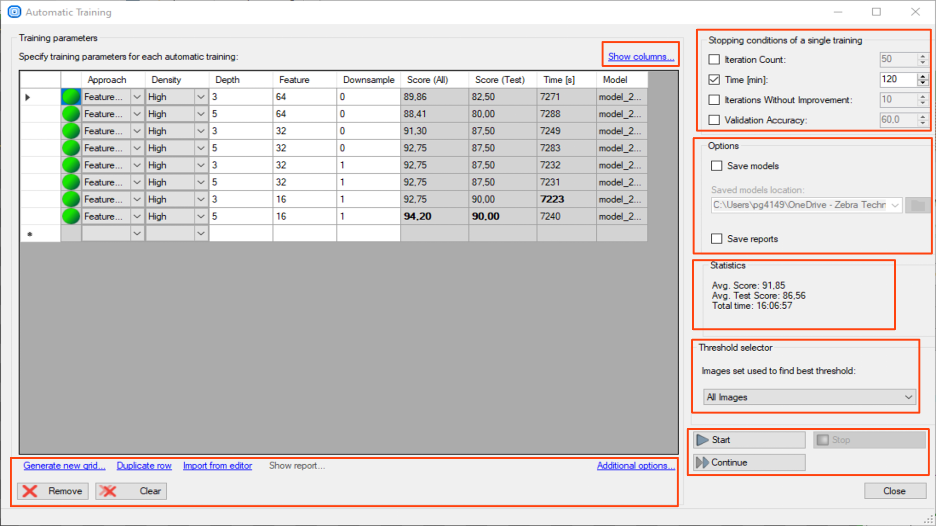
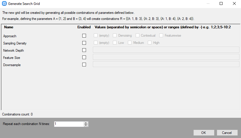
Open automatic training window button – allows you to prepare a training series for different parameters.
If you are not sure, which parameter settings will give you the best result, you can prepare a combination for each value to compare the results.
The test parameters can be prepared automatically with Generate new grid or manually entered. After setting the parameters you need to start the test.
The settings and the results are shown in the grid, one row for one model.
Show columns – hides / shows model parameters you will use in your test.
The view is common for all deep learning tools. To create an appropriate grid search, choose these parameters which are correct for the used tool (the ones you can see in Training Parameters). For DL_DetectAnomalies2 choose the network type first to see the appropriate parameters.
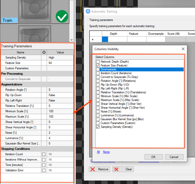
Generate new grid – prepares the search grid for the given parameters. Only parameters chosen in Show columns are available. The values should be separated with ; sign.
Duplicate rows – duplicates a training parameters configuration. If the parameters inside the row won't be modified, this model will use the same settings twice for the training.
Import from editor – copies the training parameters from Editor Window to the last search grid row.
Show report – shows the report for the chosen model (the chosen row). This option is available only if you choose Save Reports before starting the training session.
Additional options
- Export grid to CSV file – exports the grid of training parameters to a CSV file.
- Import grid from CSV file – imports the grid of training parameters from a CSV file.
Remove – removes a chosen training configuration.
Clear – clears the whole search grid.
Stopping conditions of a single training – determines when a single training stops.
- Iteration Count
- Time
- Iterations without improvement
- Validation Accuracy
Options
- Save models – saves each trained model in the defined folder.
- Save reports – saves a report for each trained model in the folder defined for saving models.
Statistics – shows statistics for all trainings.
- Avg. Score – shows average score of all trained models for all images.
- Avg. Test Score – shows average score of all trained models for test images.
- Total time – sums up time of each training.
Threshold selector – choses for which image group the best threshold is searched.
- All Images
- Test Images
Start – starts the training series with the first defined configuration.
Stop – stops the training series.
Continue – continues the stopped training series with the next configuration of the parameters.
Detecting anomalies 1
In this tool the user only needs to mark which images contain correct cases (good) or incorrect ones (bad). Training is performed on good images only. Inference can later be performed on both good and bad images to determine a suitable threshold.
1. Marking Good and Bad samples and dividing them into Test, Training and Validation data.
Click on a question mark sign to label each image in the training set as Good or Bad. Green and red icons on the right side of the training images indicate to which set the image belongs to. Alternatively, you can use Add images and mark.... Then divide the images into Train, Test or Validation by clicking on the left label on an image. Remember that all bad samples should be marked as Test.
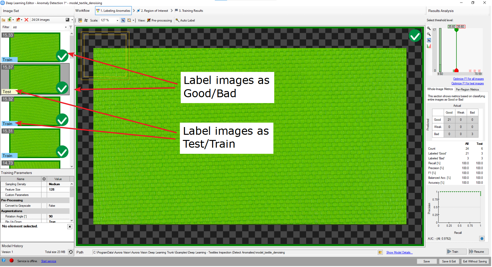
Labeled images in Deep Learning Editor.
2. Configuring augmentations
It is usually recommended to add some additional sample augmentations, especially when the training set is small. For example, the user can add additional variations in pixels intensity to prepare the model for varying lighting conditions on the production line. Refer to "Augmentation" section for detailed description of parameters: Deep Learning – Augmentation.
3. Reducing region of interest
Reduce region of interest to focus only on the important part of the image. Reducing region of interest will speed up both training and inference.
Please note that the Region of Interest in this tool is the same for each image in a training set and it cannot be adjusted individually. As a result, this Region of Interest is automatically applied during execution of a model, so a user has no impact on its size or shape in the Program Editor.
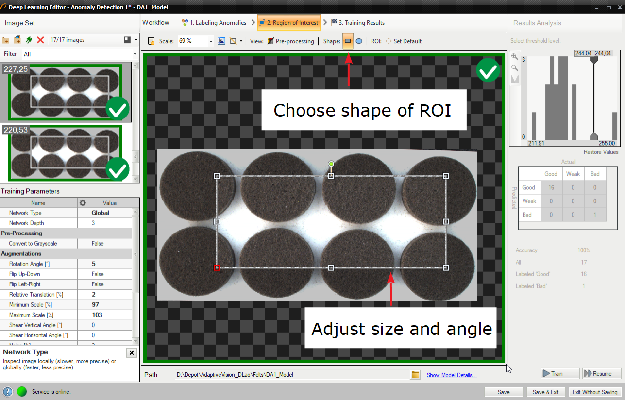
By default region of interest contains the whole image.
4. Setting training parameters
- Sampling density – determines the spatial overlap of inspection windows.
- Feature size – the width of the inspection window. In the top left corner of the editor a small rectangle visualizes the selected feature size.
- Stopping conditions – define when the training process should stop.
For more details read Deep Learning – Setting parameters.
5. Performing training
During training, two figures are successively displayed: training error and validation error. Both charts should have a similar pattern.
More detailed information is displayed on the chart below:
- current training statistics (training and validation),
- number of processed samples (depends on the number of images and feature size),
- elapsed time.
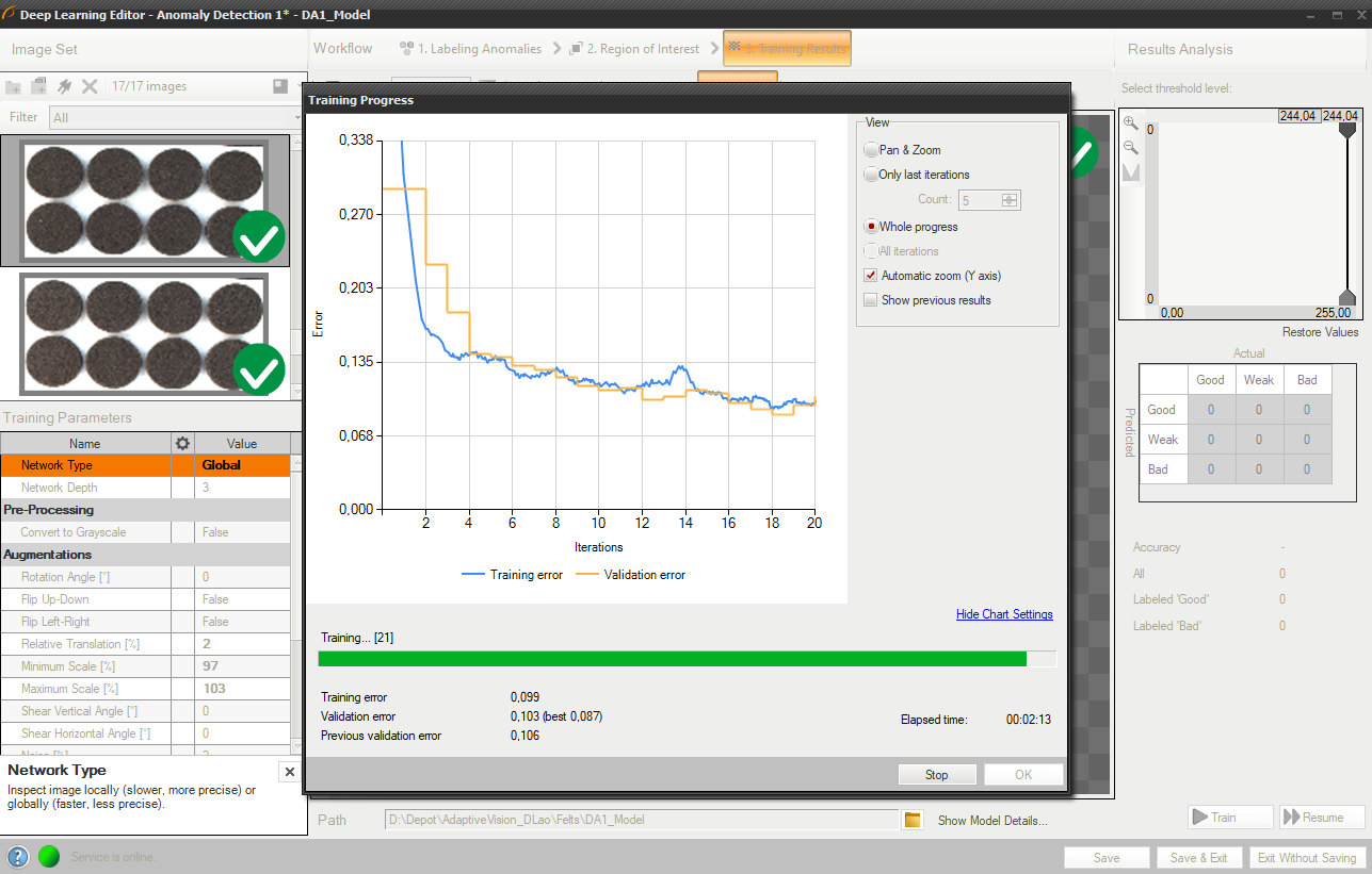
Training process consists of computing training and validation errors.
Training process can take its time depending on the selected stopping criteria and available hardware. During this time training can be finished manually anytime by clicking Stop button. If no model is present (the first training attempt) model with the best validation accuracy will be saved. Consecutive training attempts will prompt user about old model replacement.
6. Analyzing results
The window shows a histogram of sample scores and a heatmap of found defects. The right column contains a histogram of scores computed for each image in the training set. Additional statistics are displayed below the histogram.
To evaluate trained model, Evaluate: This Image or Evaluate: All Images buttons can be used. It can be useful after adding new images to the data set or after changing the area of interest.
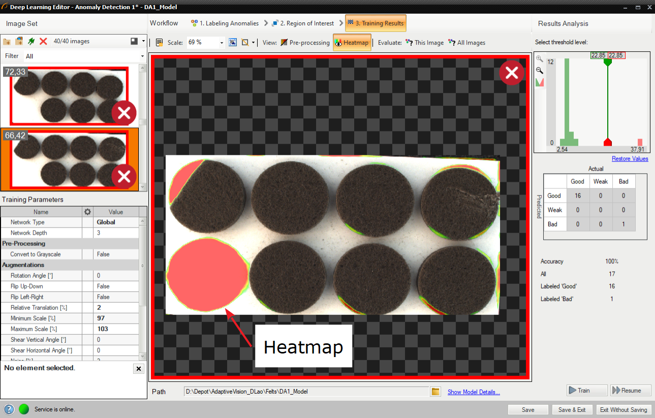
Heatmap presents the area of possible defects.
After training two border values are computed:
- Maximum good sample score (T1) – all values from 0 to T1 are marked as Good.
- Minimum bad sample score (T2) – all values greater than T2 are marked as Bad.
All scores between T1 and T2 are marked as "Low quality". Results in this range are uncertain and may be not correct. Filters contain an additional output outIsConfident which determines the values which are not in the T1-T2 range.
After evaluation additional filtering options may be used in the the list of training images.
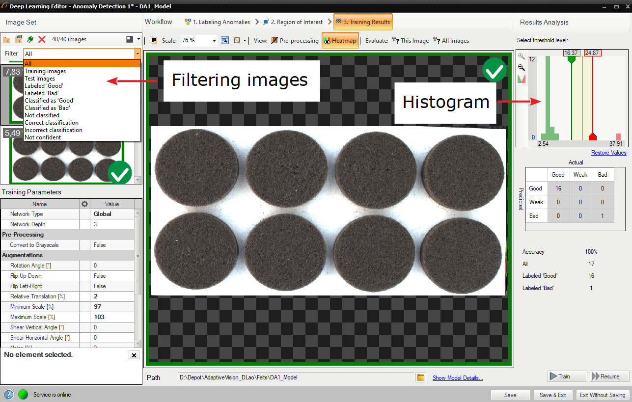
Filtering the images in the training set.
Interactive histogram tool
DetectAnomalies filters measure deviation of samples from the normal image appearances learned during the training phase. If the deviation exceeds a given threshold, the image is marked as anomalous. The suggested threshold is automatically calculated after the training phase but it can also be adjusted by the user in the Deep Learning Editor using an interactive histogram tool described below.
After the training phase, scores are calculated for every training sample and are presented in the form of a histogram; good samples are marked with green, bad samples with red bars. In the perfect case, the scores for good samples should be all lower than for bad samples and the threshold should be automatically calculated to give the optimal accuracy of the model. However, the groups may sometimes overlap because of:
- incorrectly labeled samples,
- bad Feature Size,
- ambiguous definition of the expected defects,
- high variability of the samples appearance or environmental conditions.
In order to achieve more robust threshold, it is recommended to perform training with a large number of samples from both groups. If the number of samples is limited, our software makes it possible to manually set the uncertainty area with additional thresholds (the information about the confidence of the model can be then obtained from the hidden outIsConfident filter output).
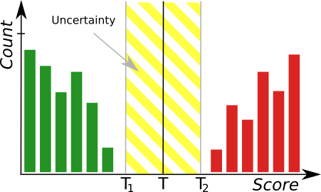
The histogram tool where green bars represent correct samples and red bars represent anomalous samples. T marks the main threshold and T1, T2 define the area of uncertainty.
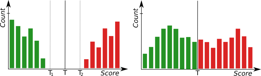
Left: a histogram presenting well-separated groups indicating a good accuracy of the model. Right: a poor accuracy of the model.
Detecting anomalies 2 (classification-based approach)
DL_DetectAnomalies2 is another filter which can be used for detecting anomalies. It is designed to solve the same problem, but in a different way. Instead of using image reconstruction techniques Anomaly Detection 2 performs one-class classification of each part of the input image.
As both tools are very similar the steps of creating a model are the same. There are only a few differences between those filters in the model parameters section. In case of DL_DetectAnomalies2 the user does not need to change iteration count and network type. Instead, it is possible to set the Model Complexity that defines the size of the resulting model. The higher the Model Complexity, the more precise the resulting heatmaps, but the larger the resulting model sizes. The Golden Template approach also features the Max Translation parameter which determines the spatial tolerance of the model.
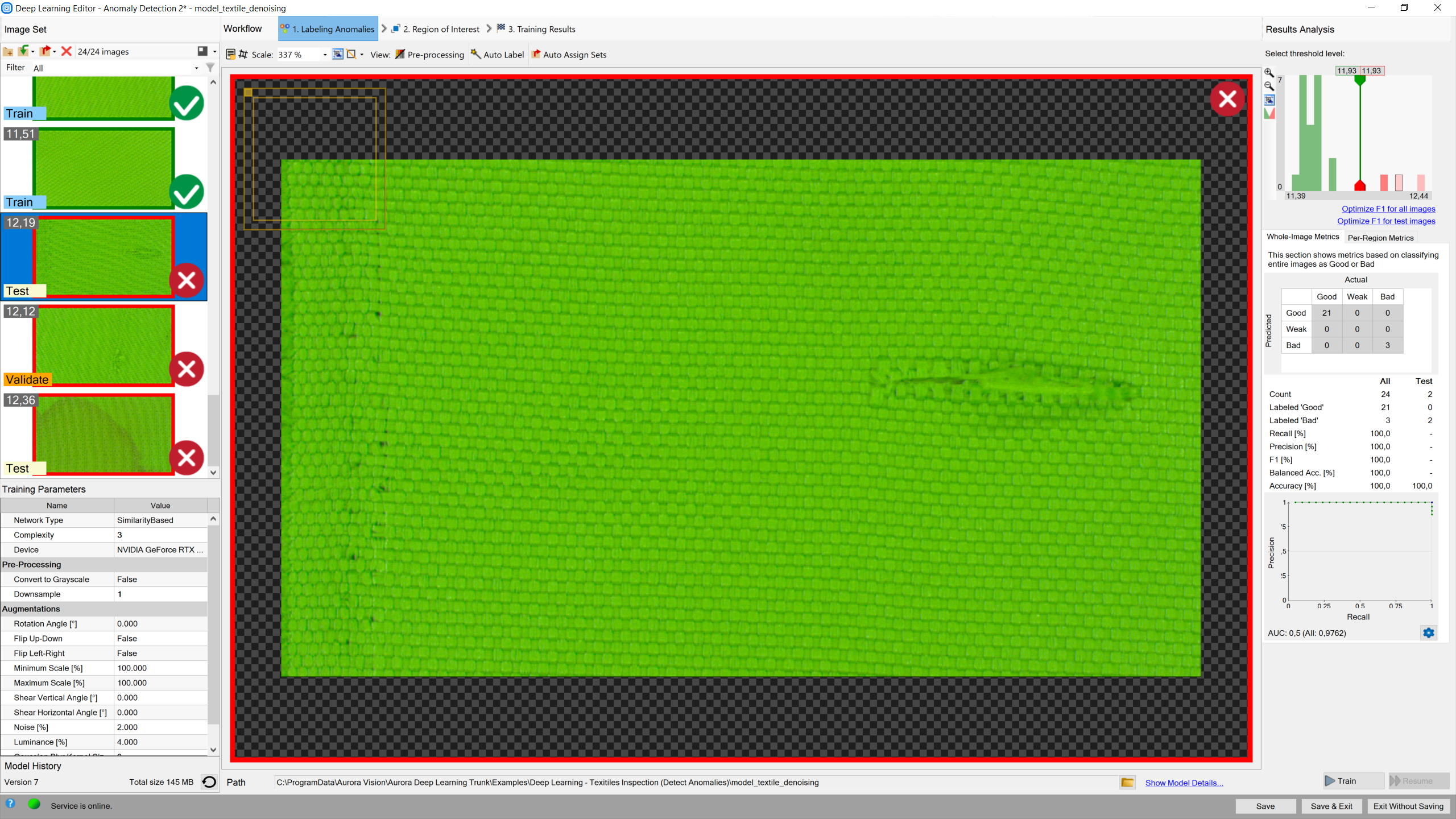
Results are marked as rectangles of either of two colors: green (classified as good) or red (classified as bad).
The resulting heatmap is usually not as accurate spatially as in case of using reconstructive anomaly detection, but the score accuracy and group separation on the histogram may be much better.
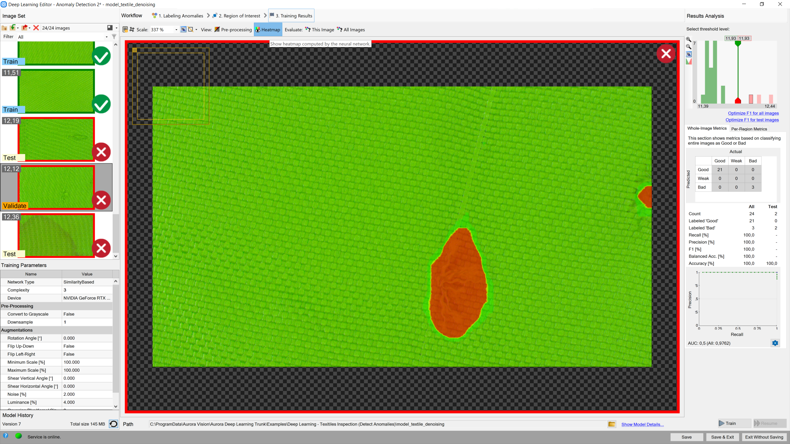
Heatmap indicates the most possible locations of defects.
Detecting features (segmentation)
In this tool the user has to define each feature class and then mark features on each image in the training set. This technique is used to find object defects like scratches or color changes, and for detecting image parts trained on a selected pattern.
1. Defining feature classes (Marking class)
First, the user has to define classes of defects. Generally, they should be features which user would like to detect on images. Multiple different classes can be defined but it is not recommended to use more than a few.
Class editor is available under sprocket wheel icon in the top bar.
To manage classes, Add, Remove or Rename buttons can be used. To customize appearance, color of each class can be changed using Change Color button.
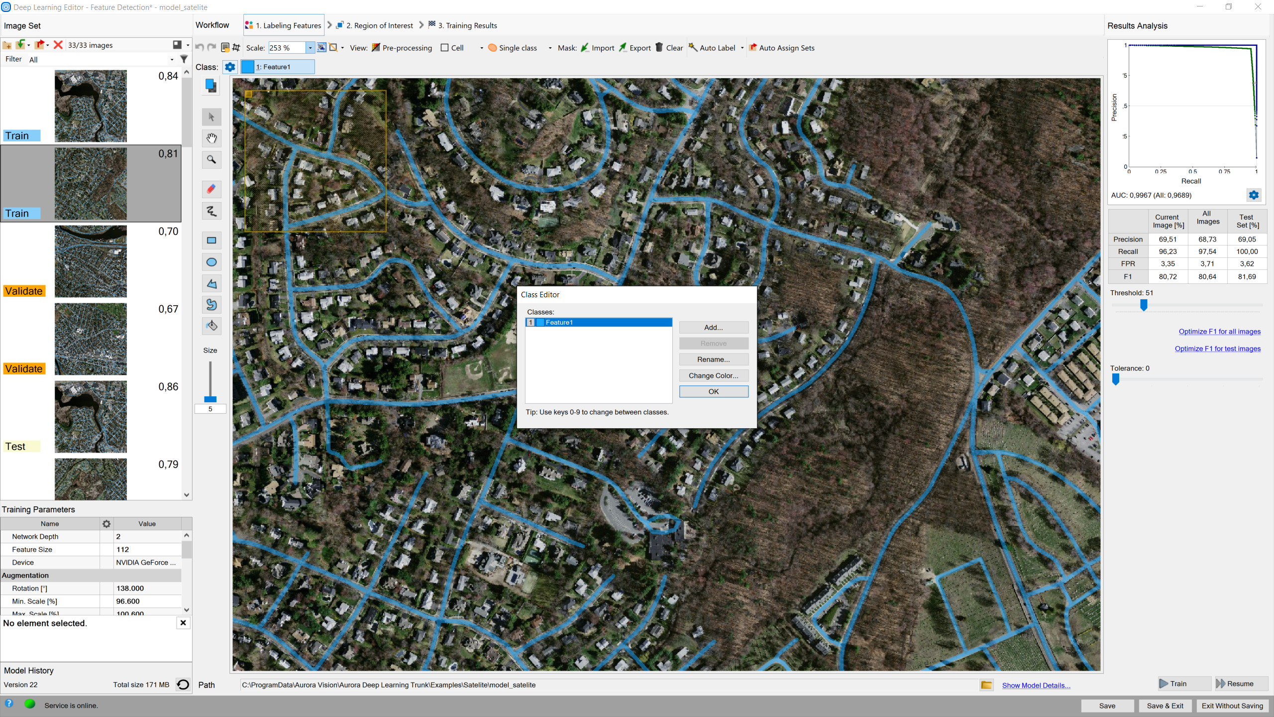
In this tool it is possible to define more classes of defects.
The current class for editing is displayed on the left, the user can select different class after click.
Use drawing tool to mark features on the input images. Tools such as Brush or Rectangle can be used for selecting features.
In addition, class masks can be imported from external files. There are buttons for Import and Export created classes so that the user can create an image of a mask automatically prior to a Deep Learning model.
The image mask should have the same size as the selected image in the input set. When importing an image mask, all non-black pixels will be included in the current mask.
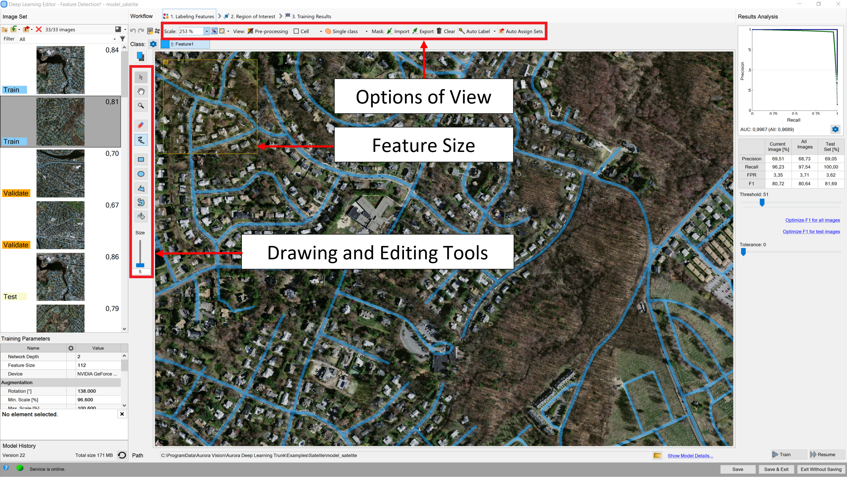
The most important features of the tool.
The user can also load multiple images and masks at the same time, using Add images and masks button.
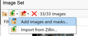
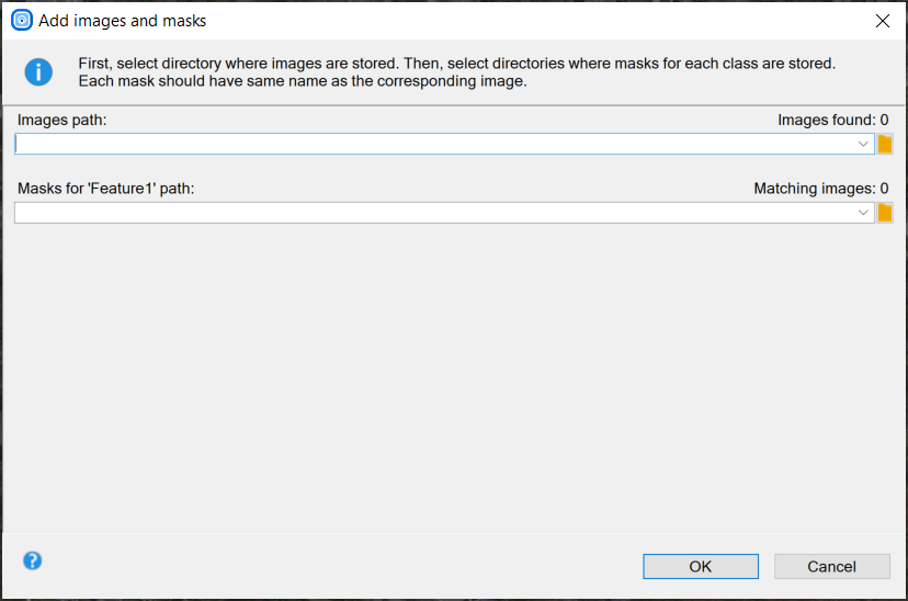
Selecting path to images and masks.
Directory containing input images should be selected first. Then, directories for each feature class can be selected below. Images and masks are matched automatically using their file names. For example, let us assume that "images" directory contains images 001.png, 002.png, 003.png; "mask_class1" directory contains 001.png, 002.png, 003.png; and "mask_class2" directory contains 001.png, 002.png, 003.png. Then "images\001.png" image will be loaded together with "mask_class1\001.png" and "mask_class2\001.png" masks.
2. Reducing region of interest
The user can reduce the input image size to speed up the training process. In many cases, number of features on an image is very large and most of them are the same. In such case the region of interest also can be reduced.
On the top bar there are tools for applying the current ROI to all images as well as for resetting the ROI.
Setting ROI.
3. Setting training parameters
- Network depth – chooses one of several predefined network architectures varying in their complexity. For bigger and more complex image patterns a higher depth might be necessary.
- Patch size – the size of an image part that will be analyzed with one pass through the neural network. It should be significantly bigger than any feature of interest, but not too big – as the bigger the patch size, the more difficult and time consuming is the training process.
- Stopping conditions – define when the training process should stop.
For more details please refer to Deep Learning – Setting parameters and Deep Learning – Augmentation.
4. Model training
The chart contains two series: training and validation score. Higher score value leads to better results.
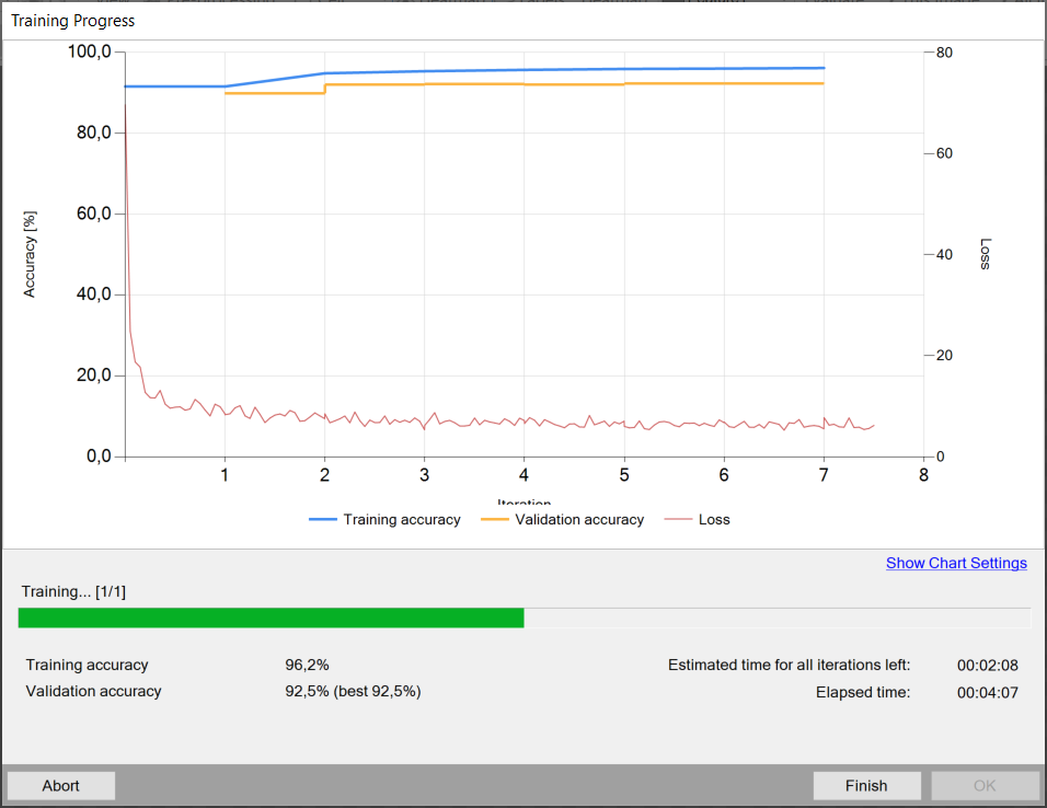
In this case training process consists of computing training and validation accuracies.
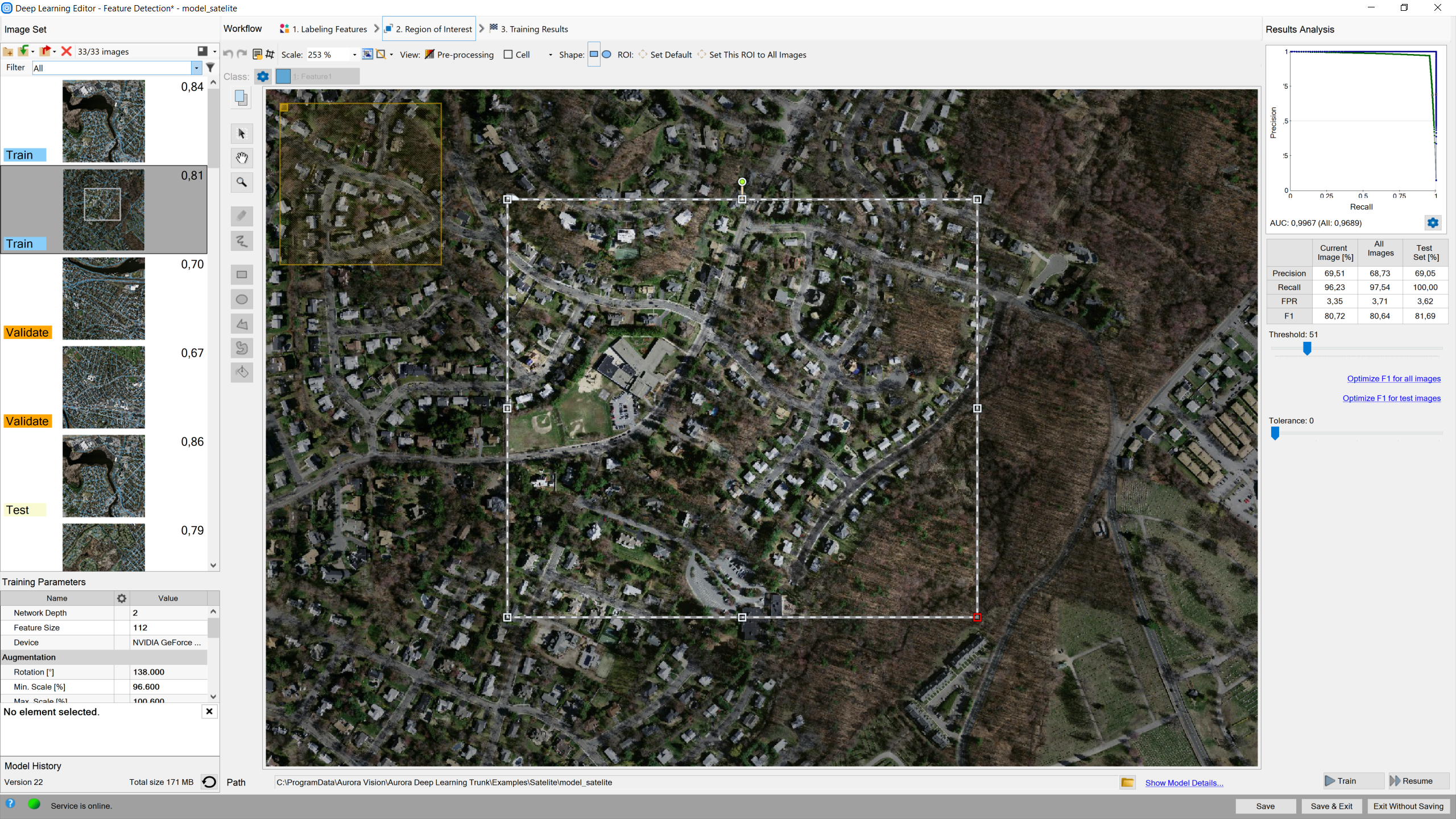
5. Result analysis
Image scores (heatmaps) are displayed in red after using the model for evaluation of the image. These scores indicate the association of a specific part of the image to the currently selected feature class.
Evaluate: This Image and Evaluate: All Images buttons can be used to classify images. It can be useful after adding new images to the data set or after changing the area of interest.
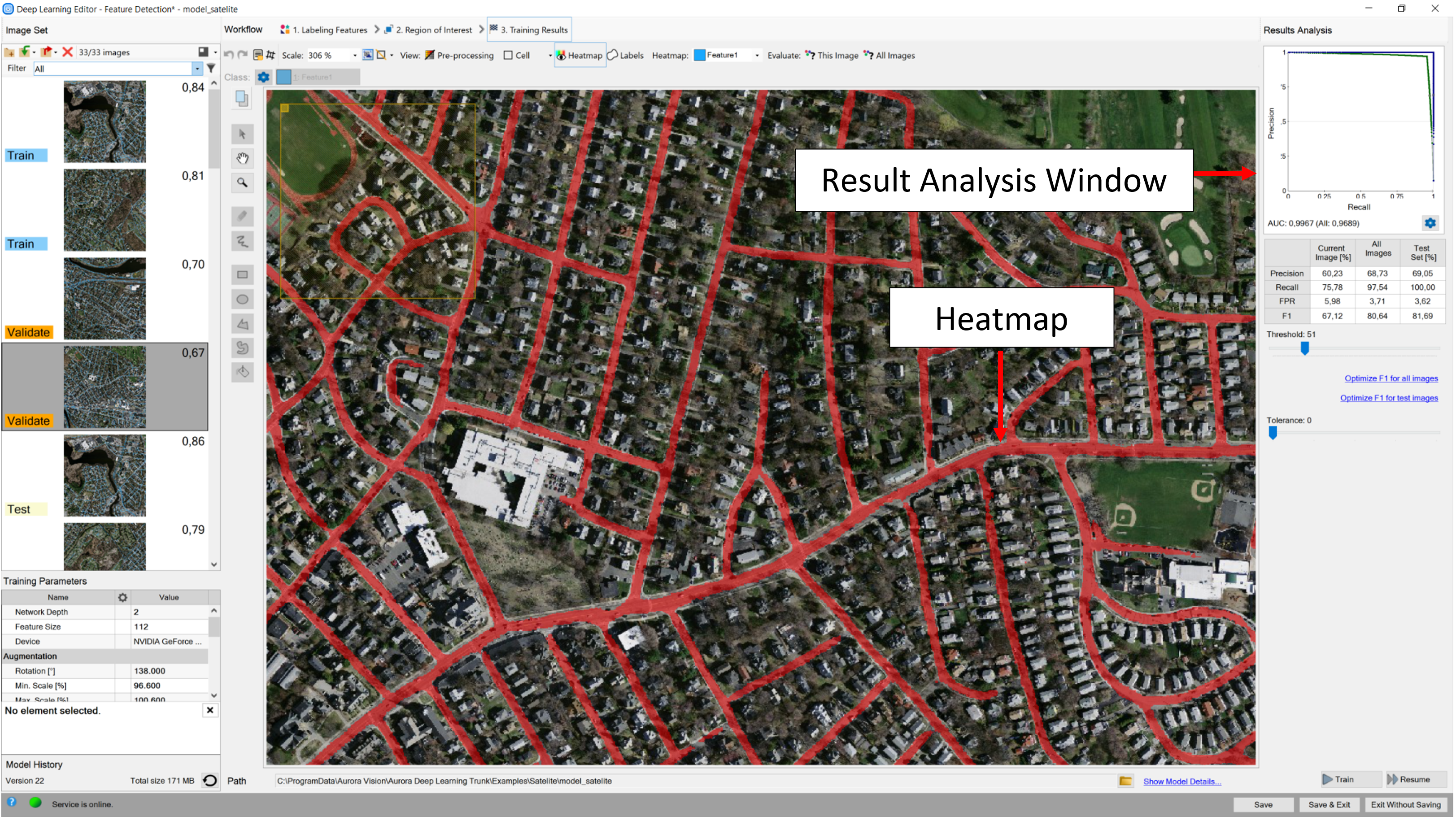
Image after classification.
In the top left corner of the editor, a green rectangle visualizes the selected patch size.
Classifying objects
In this too, the user only has to label images with respect to a desired number of classes. Theoretically, the number of classes that a user can create is infinite, but please note that you are limited by the amount of data your GPU can process. Labeled images will allow to train model and determine features which will be used to evaluate new samples and assign them to proper classes.
1. Editing number of classes
By default two classes are defined. If the problem is more complex than that, the user can edit classes and define more if needed. Once the user is ready with definition of classes, images can be labeled.
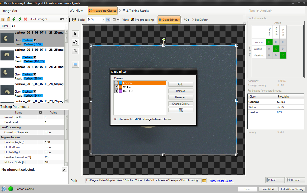
Using Class Editor.
2. Labeling samples
Labeling of samples is possible after adding training images. Each image has a corresponding drop-down list which allows for assigning a specific class. It is possible to assign a single class to multiple images by selecting desired images in Deep Learning Editor.
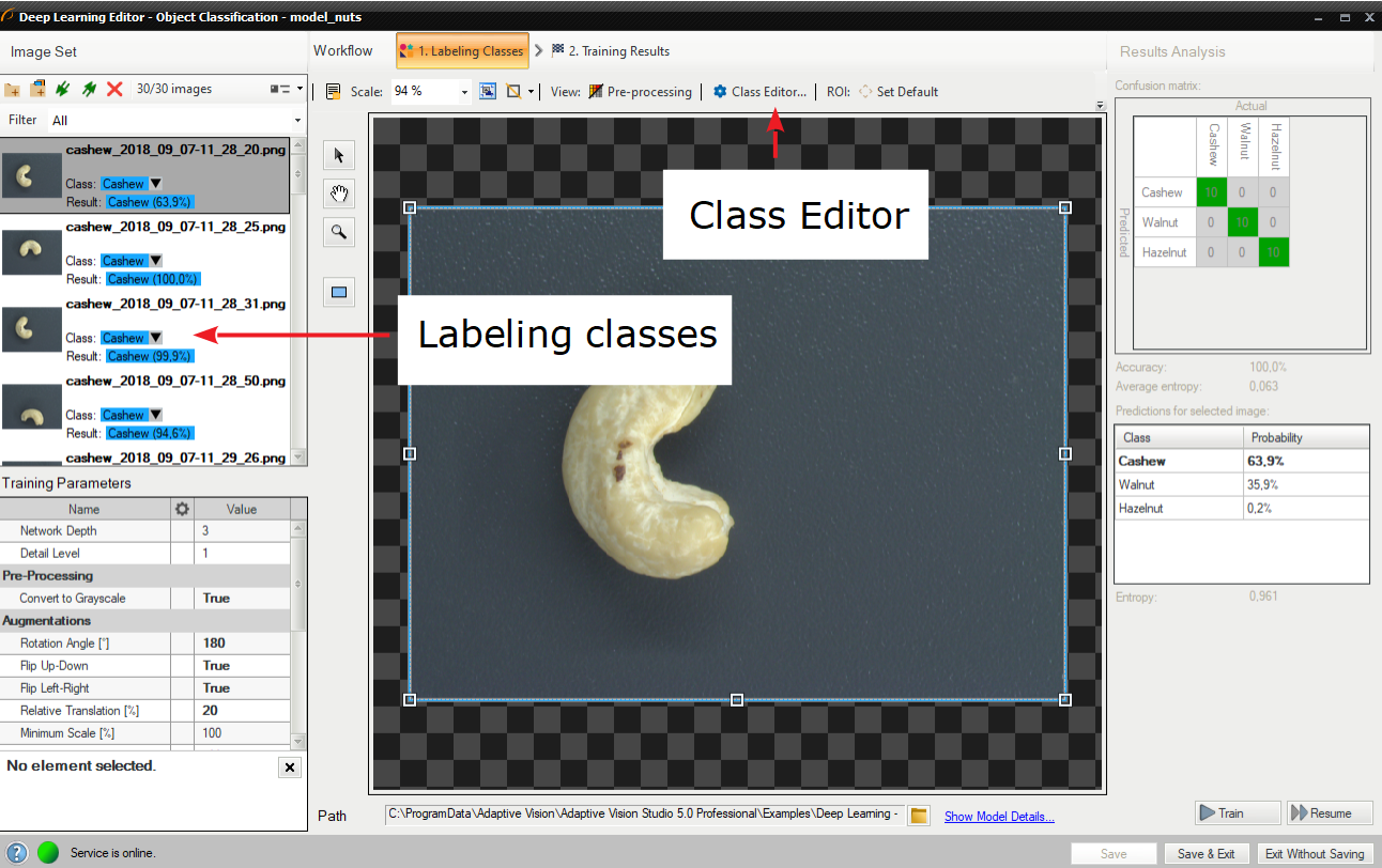
Labeling images with classes.
3. Reducing region of interest
Reduce the region of interest to focus only on the important part of the image. Reducing region of interest will speed up both training and classification. By default the region of interest contains the whole image.
To get the best classification results, use the same region of interest for training and classification.
Changed region of interest.
4. Setting training parameters
- Network depth – predefined network architecture parameter. For more complex problems higher depth might be necessary.
- Detail level – level of detail needed for a particular classification task. For majority of cases the default value of 1 is appropriate, but if images of different classes are distinguishable only by small features, increasing value of this parameter may improve classification results.
- Stopping conditions – define when the training process should stop.
For more details please refer to Deep Learning – Setting parameters and Deep Learning – Augmentation.
5. Performing training
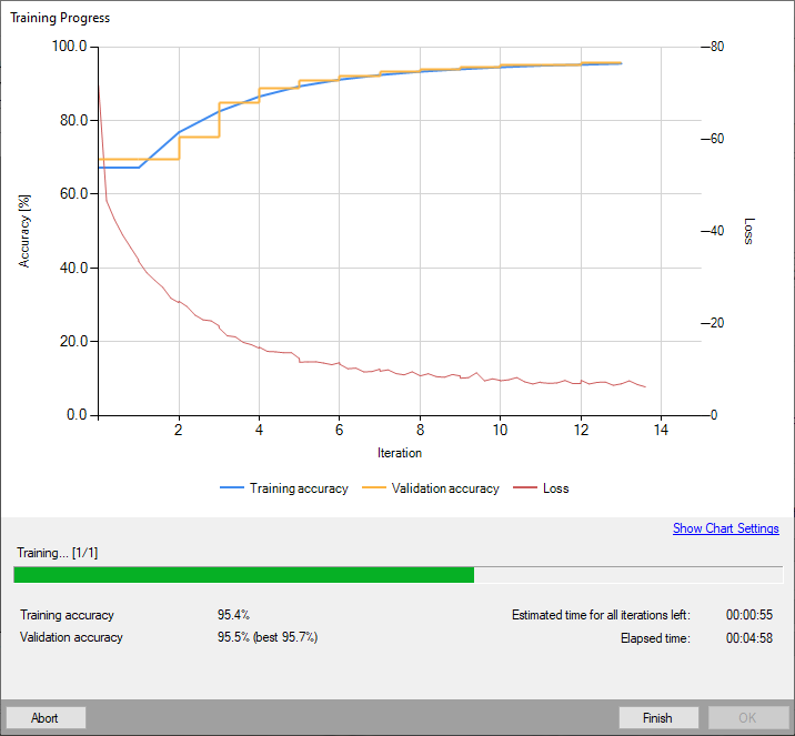
During training two series are visible: training accuracy and validation accuracy. Both charts should have a similar pattern.
More detailed information is displayed below the chart:
- current training statistics (training and validation accuracy),
- number of processed samples (depends on the number of images),
- elapsed time.
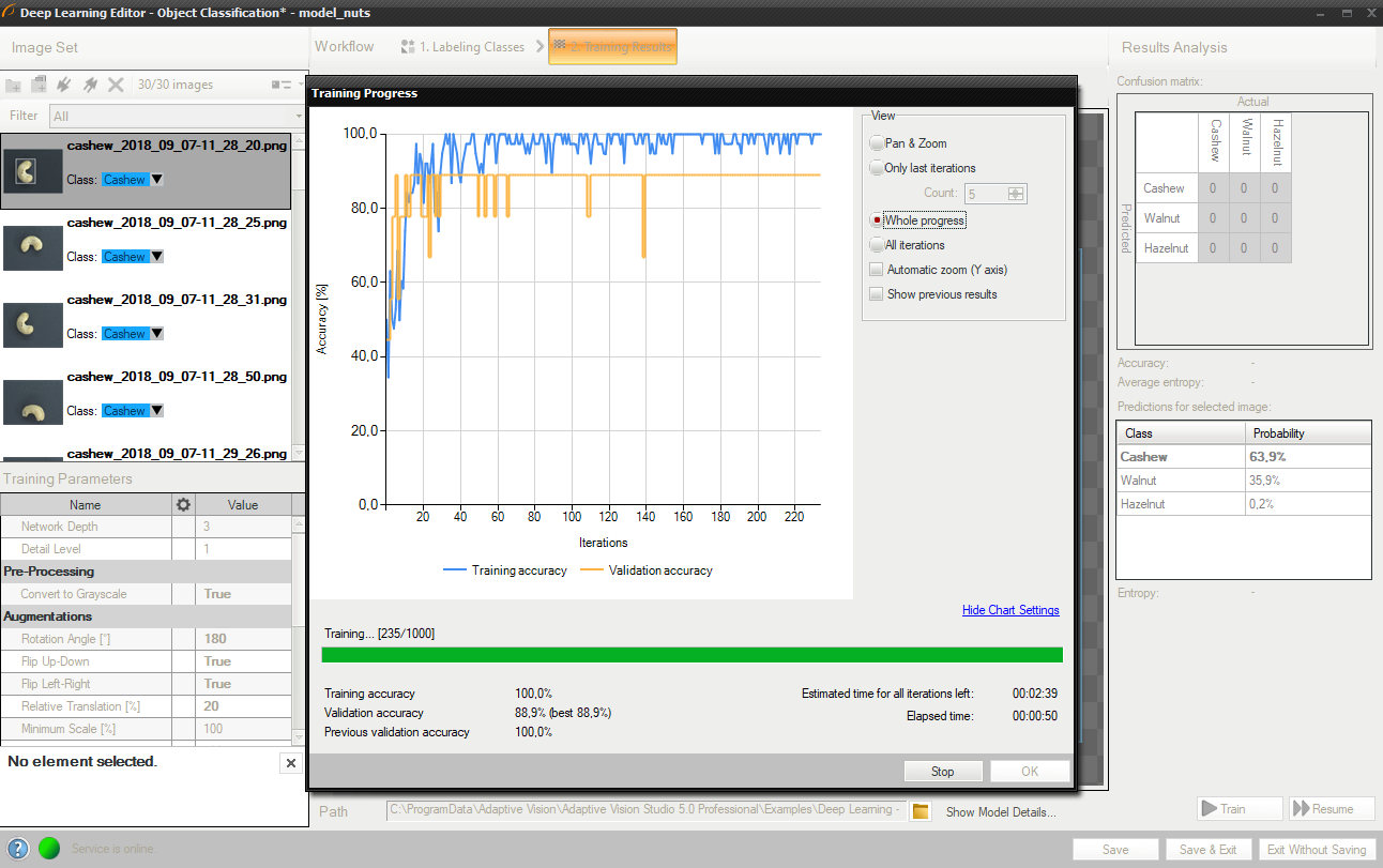
Training object classification model.
Training process can take a couple of minutes or even longer. It can be manually finished if needed. The final result of one training is one of the partial models that achieved the highest validation accuracy (not necessarily the last one). Consecutive training attempts will prompt the user whether to save a new model or keep the old one.
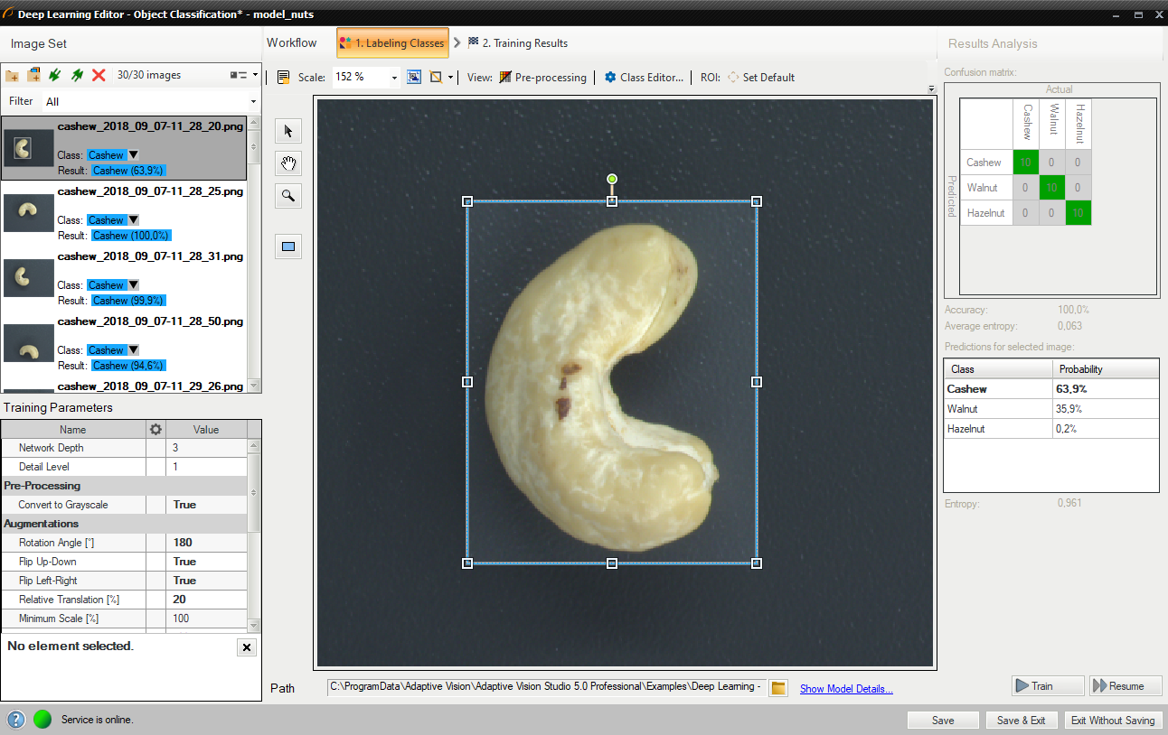
6. Analyzing results
The window shows a confusion matrix which indicates how well the training samples have been classified.
The image view contains a heatmap which indicates which part of the image contributed the most to the classification result.
Evaluate: This Image and Evaluate: All Images buttons can be used to classify training images. It can be useful after adding new images to the data set or after changing the area of interest.
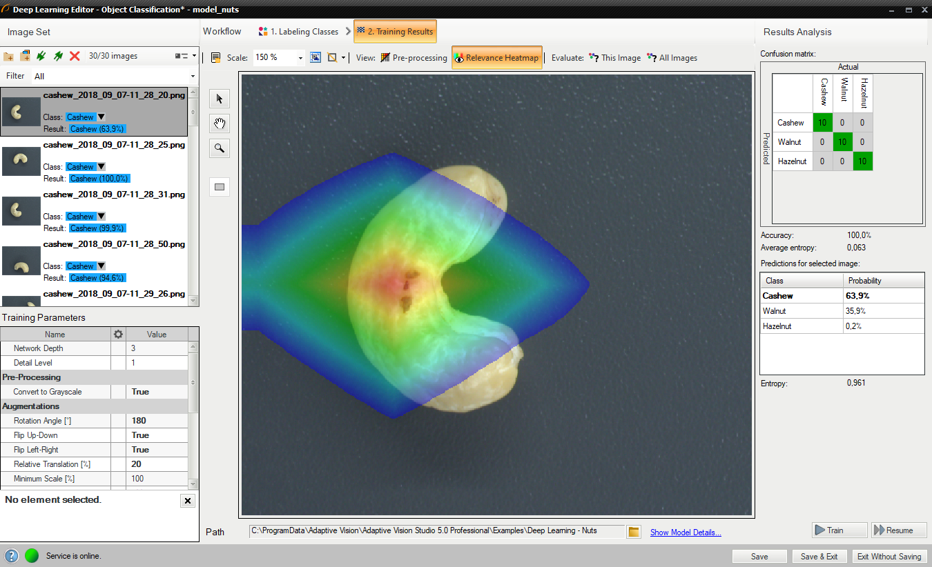
Confusion matrix and class assignment after the training.
Sometimes it is hard to guess the right parameters in the first attempt. The picture below shows confusion matrix that indicates inaccurate classification during the training (left).
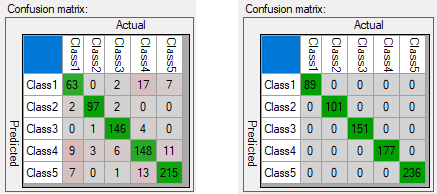
Confusion matrices for model that needs more training (left) and for model well trained (right).
It is possible that confusion matrix indicates that trained model is not 100% accurate with respect to training samples (numbers assigned exclusively on main diagonal represent 100% accuracy). User needs to properly analyze this data, and use to his advantage.
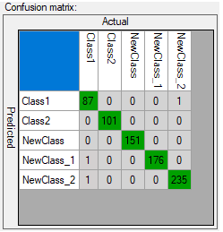
Confusion matrix indicating good generalization.
Too many erroneous classifications indicate poor training. Few of them may indicate that model is properly focused on generalization rather than exact matching to training samples (possible overfitting). Good generalization can be achieved if images used for training are varied (even among single class). If provided data is not varied within classes (user expects exact matching), and still some images are classified outside main diagonal after the training, user can:
- increase the network depth,
- prolong training by increasing number of iterations,
- increase amount of data used for training,
- use augmentation,
- increase the detail level parameter.
Segmenting instances
In this tool a user needs to draw regions (masks) corresponding to the objects in the scene and specify their classes. These images and masks are used to train a model which then in turn is used to locate, segment and classify objects in the input images.
1. Defining object classes
First, a user needs to define classes of objects that the model will be trained on and that later it will be used to detect. Instance segmentation model can deal with single as well as multiple classes of objects.
Class editor is available under the Class Editor button.
To manage classes, Add, Remove or Rename buttons can be used. To customize appearance, color of each class can be changed using the Change Color button.
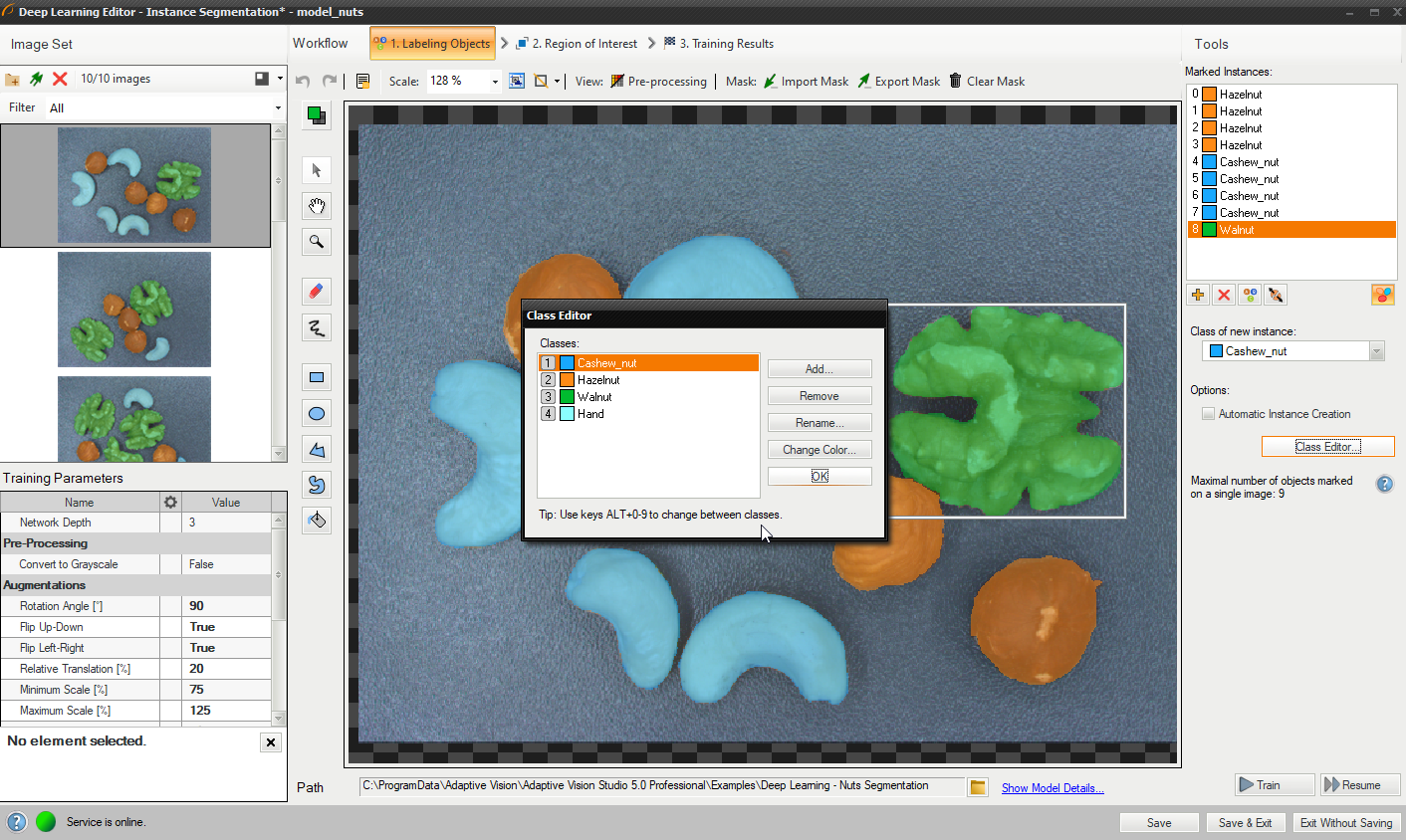
Using Class Editor.
2. Labeling objects
After adding training images and defining classes a user needs to draw regions (masks) to mark objects in images.
To mark an object the user needs to select a proper class in the Current Class drop-down menu and click the Add Instance button (green plus). Alternatively, for convenience of labeling, it is possible to apply Automatic Instance Creation which allows a user to draw quickly masks on multiple objects in the image without having to add a new instance every time.
Use drawing tool to mark objects on the input images. Multiple tools such as brush and shapes can be used to draw object masks. Masks are the same color as previously defined for the selected classes.
The Marked Instances list in the top left corner displays a list of defined objects for the current image. If an object does not have a corresponding mask created in the image, it is marked as "(empty)". When an object is selected, a bounding box is displayed around its mask in the drawing area. Selected object can be modified in terms of a class (Change Class button) as well as a mask (by simply drawing new parts or erasing existing ones). Remove Instance button (red cross) allows to completely remove a selected object.
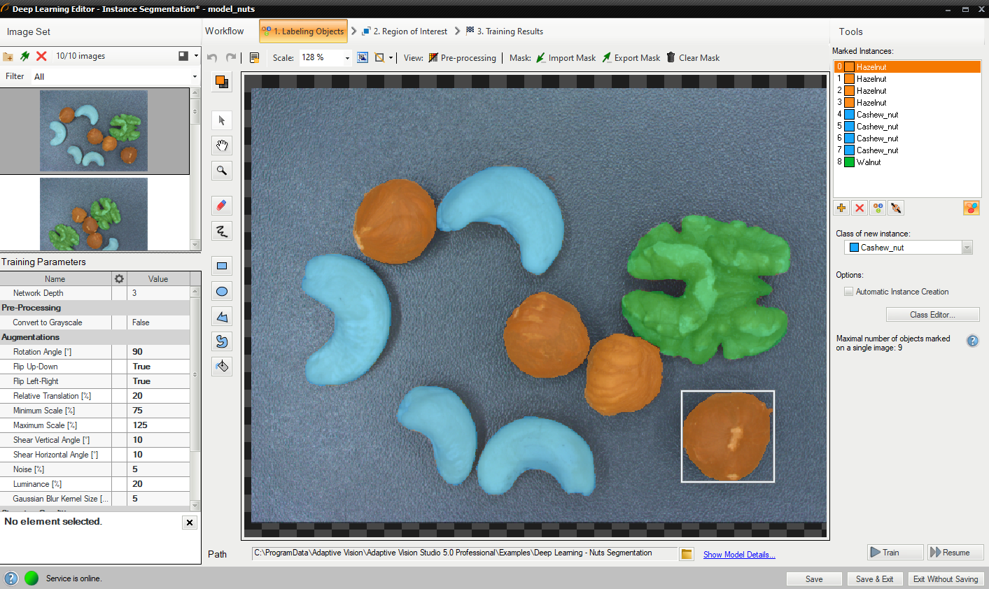
Labeling objects.
3. Reducing region of interest
Reduce region of interest to focus only on the important part of the image. By default region of interest contains the whole image.
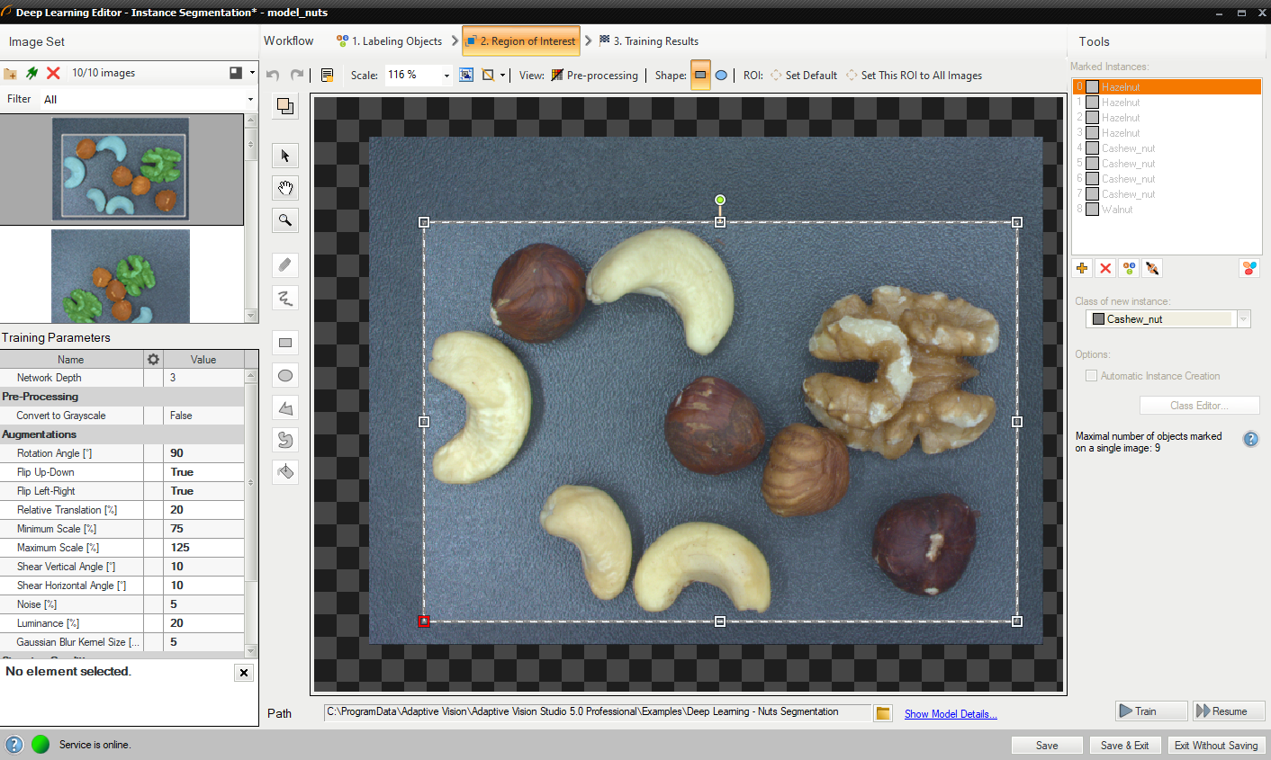
Changing region of interest.
4. Setting training parameters
- Network depth – predefined network architecture parameter. For more complex problems higher depth might be necessary,
- Stopping conditions – define when the training process should stop.
For more details read Deep Learning – Setting parameters.
Details regarding augmentation parameters. Deep Learning – Augmentation
5. Performing training
During training two main series are visible: training error and validation error. Both charts should have a similar pattern. If a training was run before the third series with previous validation error is also displayed.
More detailed information is displayed below the chart:
- current iteration number,
- current training statistics (training and validation error),
- number of processed samples,
- elapsed time.
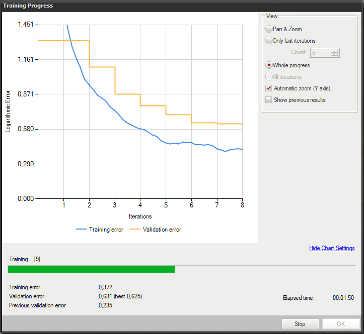
Training instance segmentation model.
Training may be a long process. During this time, training can be stopped. If no model is present (first training attempt) model with best validation accuracy will be saved. Consecutive training attempts will prompt a user whether to replace the old model.
6. Analyzing results
The window shows the results of instance segmentation. Detected objects are displayed on top of the images. Each detection consists of following data:
- class (identified by a color),
- bounding box,
- model-generated instance mask,
- confidence score.
Evaluate: This Image and Evaluate: All Images buttons can be used to perform instance segmentation on the provided images. It can be useful after adding new images to the data set or after changing the area of interest.
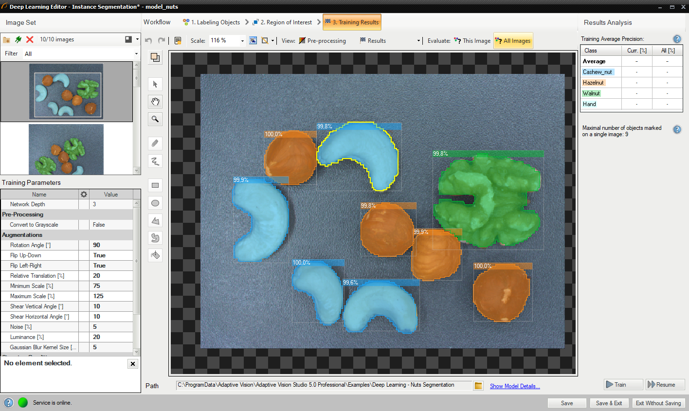
Instance segmentation results visualized after the training.
Instance segmentation is a complex task therefore it is highly recommended to use data augmentations to improve network's ability to generalize learned information. If results are still not satisfactory the following standard methods can be used to improve model performance:
- providing more training data,
- increasing number of training iterations,
- increasing the network depth.
Locating points
In this tool the user defines classes and marks key points in the image. This data is used to train a model which then is used to locate and classify key points in images.
1. Defining classes
First, a user needs to define classes of key points that the model will be trained on and later used to detect. Point location model can deal with single as well as multiple classes of key points. If the size of your classes differs greatly, it is better to prepare two, or more, different models than one.
Class editor is available under the Class Editor button.
To manage classes, Add, Remove or Rename buttons can be used. Color of each class can be changed using Change Color button.
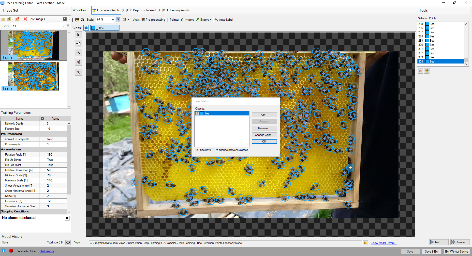
Using Class Editor.
2. Marking key points
After adding training images and defining classes a user needs to mark points in images.
To mark an object a user needs to select a proper class in the Current Class drop-down menu and click the Add Point button. Points have the same color as previously defined for the selected class.
The Selected Points list in the top rigth corner displays a list of defined points for the current image. A point can be selected either from the list of directly on the image area. A selected point can be moved, removed (Remove Point button) or has its class changed (Change Class button).
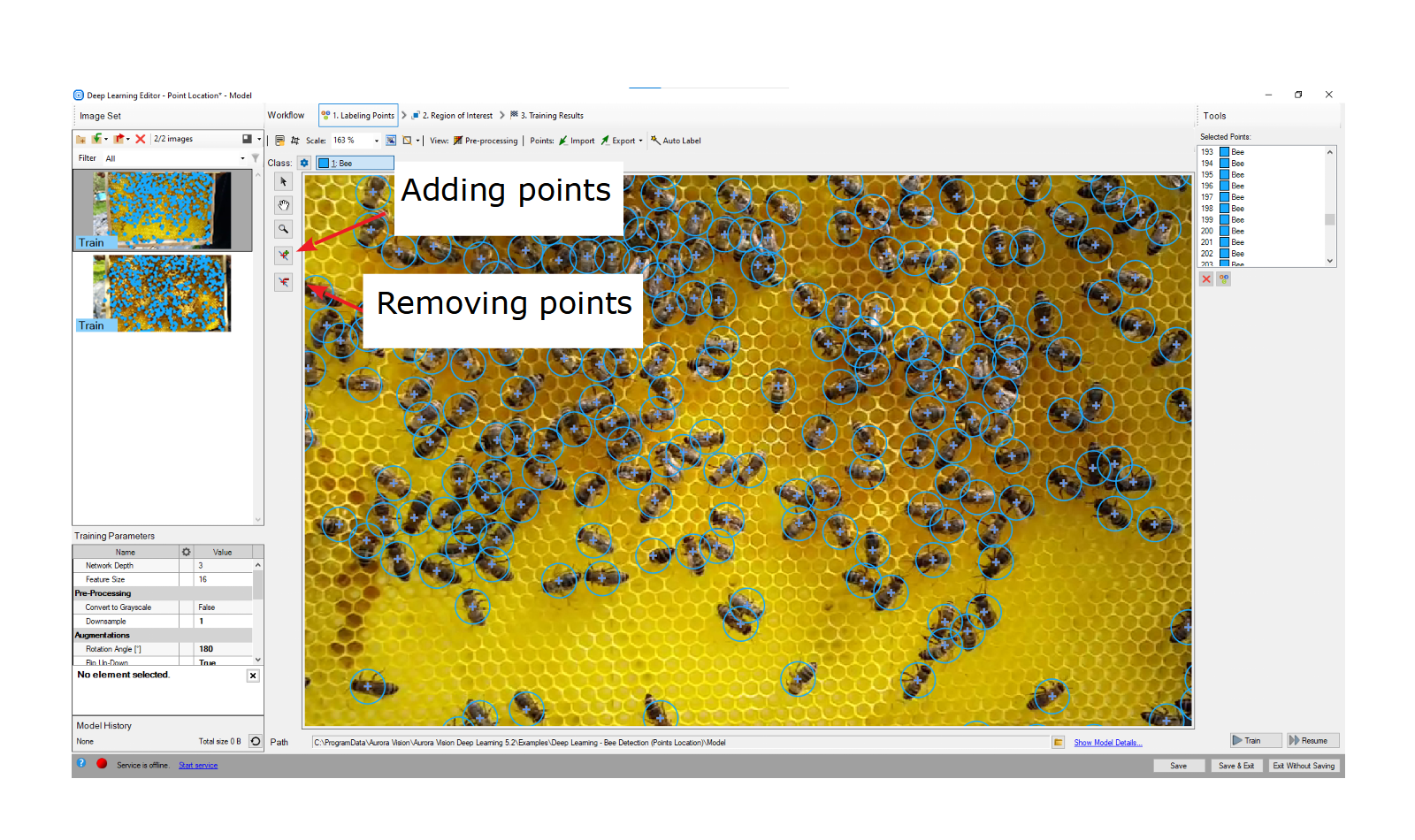
Marking points.
3. Reducing region of interest
Reduce region of interest to focus only on the important part of the image and to speed up the training process. By default region of interest contains the whole image.
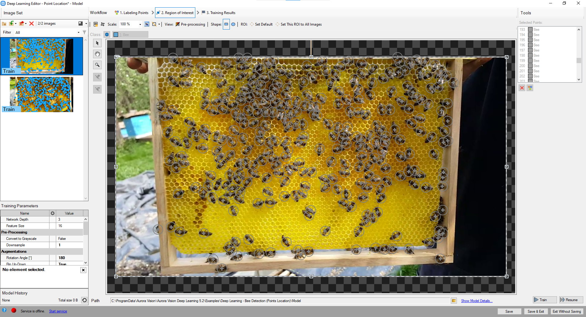
Changing region of interest.
4. Setting training parameters
- Network depth – predefined network architecture parameter. For more complex problems higher depth might be necessary.
- Feature size – the size of an small object or of a characteristic part. If images contain objects of different scales, it is recommended to use feature size slightly larger than the average object size, although it may require experimenting with different values to achieve optimal results.
- Stopping conditions – define when the training process should stop.
For more details read Deep Learning – Setting parameters.
Details regarding augmentation parameters. Deep Learning – Augmentation
5. Performing training
During training, three main series are visible: training error, validation error and training loss. All charts should have a similar pattern.
More detailed information is displayed below the chart:
- current iteration number,
- current training statistics (training and validation error),
- number of processed samples,
- elapsed time.
Training point location model.
Training may be a long process. During this time, training can be stopped. If no model is present (first training attempt) model with best validation accuracy will be saved. Consecutive training attempts will prompt user whether to replace the old model.
6. Analyzing results
The window shows results of point location. Detected points are displayed on top of the images. Each detection consists of following data:
- visualized point coordinates,
- class (identified by a color),
- confidence score.
Evaluate: This Image and Evaluate: All Images buttons can be used to perform point location on the provided images. It may be useful after adding new training or test images to the data set or after changing the area of interest.
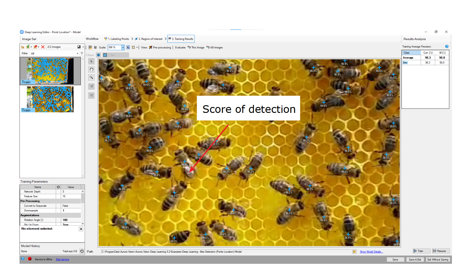
Point location results visualized after the training.
It is highly recommended to use data augmentations (appropriate to the task) to improve network's ability to generalize learned information. If results are still not satisfactory the following standard methods can be used to improve model performance:
- changing the feature size,
- providing more training data,
- increasing number of training iterations,
- increasing the network depth.
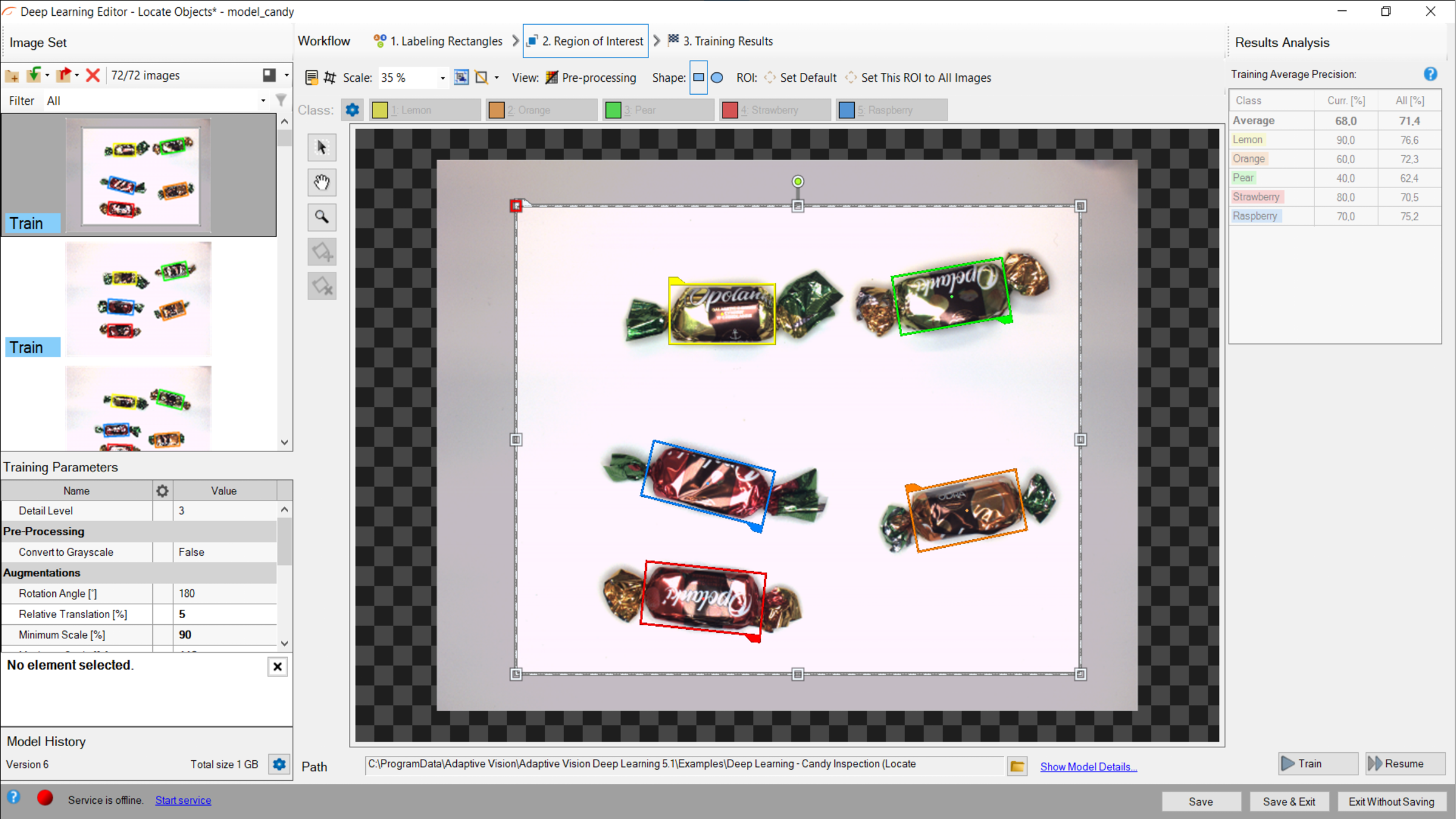
Locating objects
In this tool a user needs to draw rectangles bounding the objects in the scene and specify their classes. These images and rectangles are used to train a model to locate and classify objects in the input images. This tool doesn't require from a user to mark the objects as precisely as it is required for segmenting instances.
1. Defining classes
First, a user needs to define classes of objects that the model will be trained on and later used to detect. Object location model can deal with single as well as multiple classes of objects.
Class editor is available under the Class Editor button.
To manage classes, Add, Remove or Rename buttons can be used. Color of each class can be changed using Change Color button.
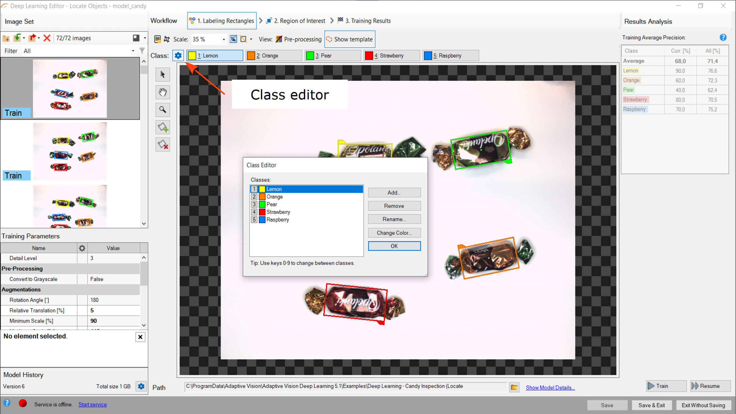
Using Class Editor.
2. Marking bounding rectangles
After adding training images and defining classes a user needs to mark rectangles in images.
To mark an object a user needs to click on a proper class from the Class Toolbar and click the Creating Rectangle button. Rectangles have the same color as previously defined for the selected class.
A rectangle can be selected directly on the image area. A selected rectangle can be moved, rotated and resized to fit it to the object, removed (Remove Region button) or has its class changed (Right click on the rectangle » Change Class button).
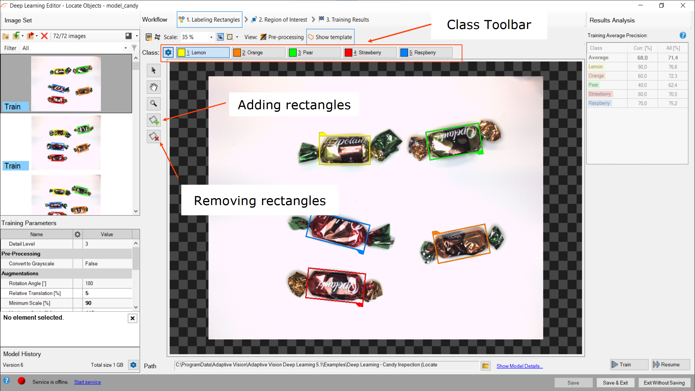
Marking rectangles.
3. Reducing region of interest
Reduce region of interest to focus only on the important part of the image and to speed up the training process. By default region of interest contains the whole image.
Changing region of interest.
4. Setting training parameters
- Detail level – level of detail needed for a particular classification task. For majority of cases the default value of 3 is appropriate, but if images of different classes are distinguishable only by small features, increasing value of this parameter may improve classification results.
- Stopping conditions – define when the training process should stop.
For more details read Deep Learning – Setting parameters.
Details regarding augmentation parameters. Deep Learning – Augmentation
5. Performing training
During training, two main series are visible: training error and validation error. Both charts should have a similar pattern. If a training was run before the third series with previous validation error is also displayed.
More detailed information is displayed below the chart:
- current iteration number,
- current training statistics (training and validation error),
- number of processed samples,
- elapsed time.
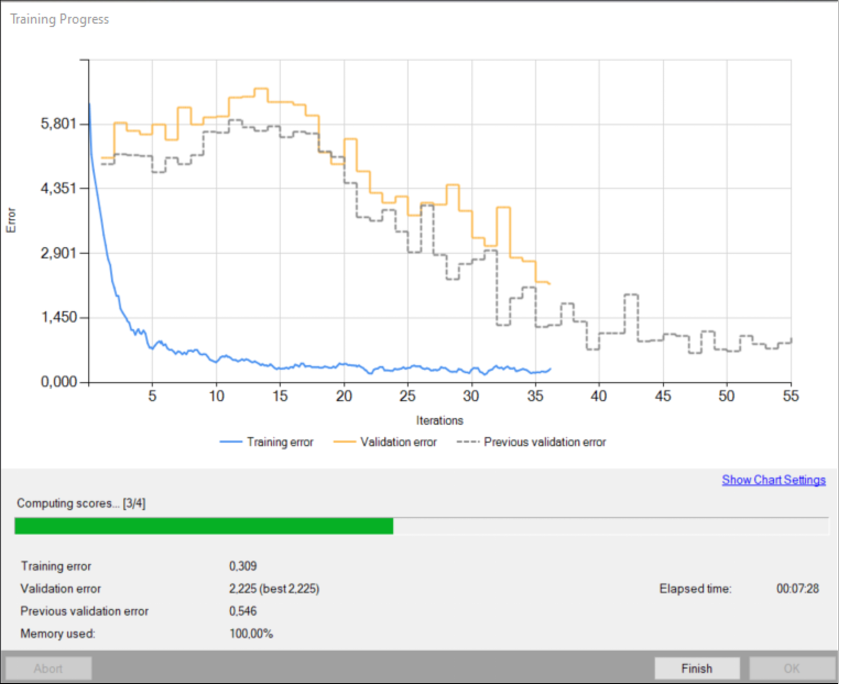
Training object location model.
Training may be a long process. During this time, training can be stopped. If no model is present (first training attempt) model with best validation accuracy will be saved. Consecutive training attempts will prompt user whether to replace the old model.
6. Analyzing results
The window shows results of object location. Detected rectangles are displayed around the objects. Each detection consists of following data:
- visualized rectangle (object) coordinates,
- class (identified by a color),
- confidence score.
Evaluate: This Image and Evaluate: All Images buttons can be used to perform object location on the provided images. It may be useful after adding new training or test images to the data set or after changing the area of interest.
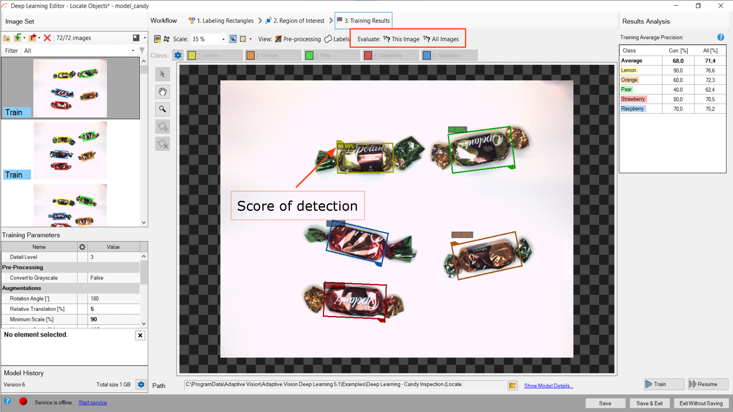
Object location results visualized after the training.
It is highly recommended to use data augmentations (appropriate to the task) to improve network's ability to generalize learned information. If results are still not satisfactory the following standard methods can be used to improve model performance:
- changing the detail level,
- providing more training data,
- increasing number of training iterations or extending the duration of the training.
Tips and tricks
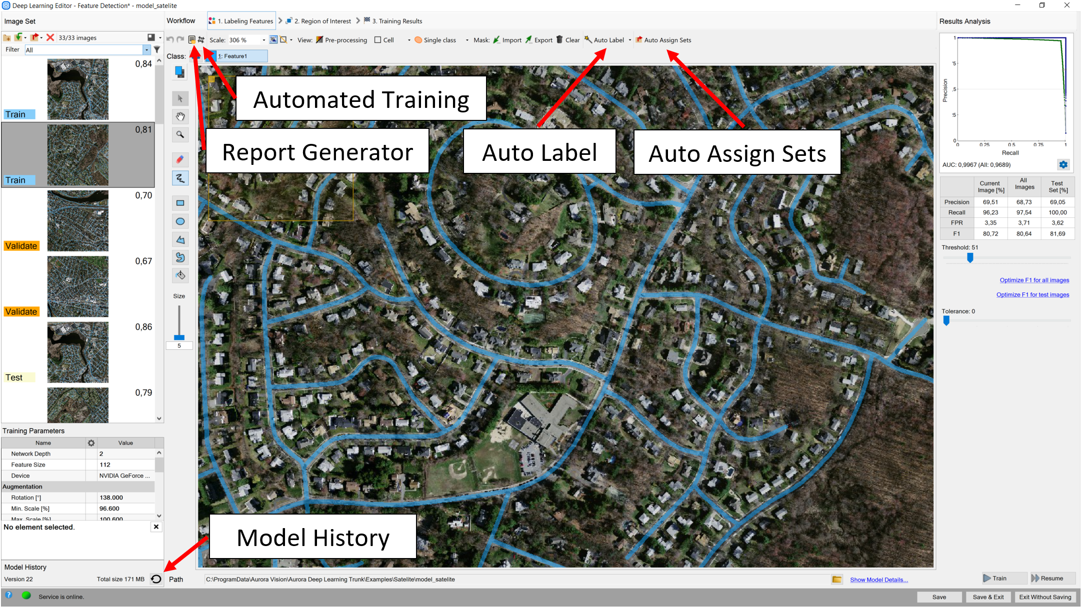
Location of useful functions
Auto label
It is a helpful feature when operating on bigger datasets, when a lot of labeling is necessary. First you need to properly label 2 images (10 is recommended) and train the model with them. If the results are satisfactory, you can add more images to your training set, select them all and press Auto Label in the Deep Learning Editor.
For supervised models the operations needs to be performed for each class you have. For unsupervised models you should do it once. Remember to always check if the masks are properly selected and correct any mistakes before continuing the training.
Auto assign sets
As of version 5.4, some of the tools may require Validation set for the training. If you are not sure which images should be picked, you can press Auto Assign Sets button. That way, from your training set, some validation images will be chosen randomly.
Model history
It is possible to access previously trained models. You can do so by pressing the looped arrow icon in the bottom left corner of the Deep Learning Editor. If you right click on a selected model, you will be able to select it instead of the current one. From that level it is also possible to remove the models you do not need.
Report generator
It is possible to generate a report of currently used model and view it, as long as the path to the images remains unchanged. To do so, simply press the report button in the editor and specify the location that you want it to be saved to.
Automated Training
For the tutorial on this tool, refer to the Automated Training section in this article.See also:
- Machine Vision Guide: Deep Learning – Deep Learning technique overview,
- Deep Learning Installation – installation and configuration of Aurora Vision Deep Learning.
| Previous: Working with 3D data | Next: Managing Workspaces |